
14.14 A person by the name of Huebscher developed a relationship between the
equivalent size of round ducts (in air-conditioning applications) and the
rectangular ducts according to:
25.0
625.0
)(
)(
3.1 ba
ab
D
where
D = diameter of equivalent circular duct (mm)
a = dimension of one side of the rectangular duct (mm)
b = the other dimension of the rectangular duct (mm)
Using Excel, create a table that shows the relationship between the circular and
the rectangular duct, similar to the one shown in the accompanying table.
Length of one side of
Rectangular Duct (length
a
)
,
mm
L
ength
b
100
125
150
175
200
400
207
450
500
550
600
191
14.15 A Pitot tube is a device commonly used in a wind tunnel to measure the speed of
the air flowing over a model. The air speed is measured from the following
equation:
d
P
V2
Where
V = air speed (m/s)
Pd = dynamic pressure (Pa)
= density of air (1.23 kg/m3)
Using Excel, create a table that shows the air speed for the range of dynamic
pressure of 500 Pa to 800 Pa. Use increments of 50 Pa.
SOLUTION
dynamic pressure (Pa)
air speed (m/s)
500
28.5
550
29.9
600
31.2
650
32.5
700
33.7
750
34.9
800
36.1
14.16 Use Excel to solve Example 7.1. Recall we applied the trapezoidal rule to
determine the area of the shape given.
SOLUTION
Area (in.2)
ybottom
192
14.17 We will discuss engineering economics in Chapter 20. Using Excel, create a
table that can be used to look up monthly payments on a car loan for a period of
five years. The monthly payments are calculated from:
1)
1200
1(
)
1200
1)(
1200
(
60
60
i
ii
PA
where
A = monthly payments in dollars
P = the loan in dollars
i = interest rate, e.g. 7, 7.5, . . ., 9
Interest rate
Loan
7
7.5
8
8.5
9
10,000
15,000
20,000
25,000
SOLUTION
Loan
7.0
7.5
8.0
8.5
9.0
10000
198.01
200.38
202.76
205.17
207.58
15000
297.02
300.57
304.15
307.75
311.38
20000
396.02
400.76
405.53
410.33
415.17
25000
495.03
500.95
506.91
512.91
518.96
193
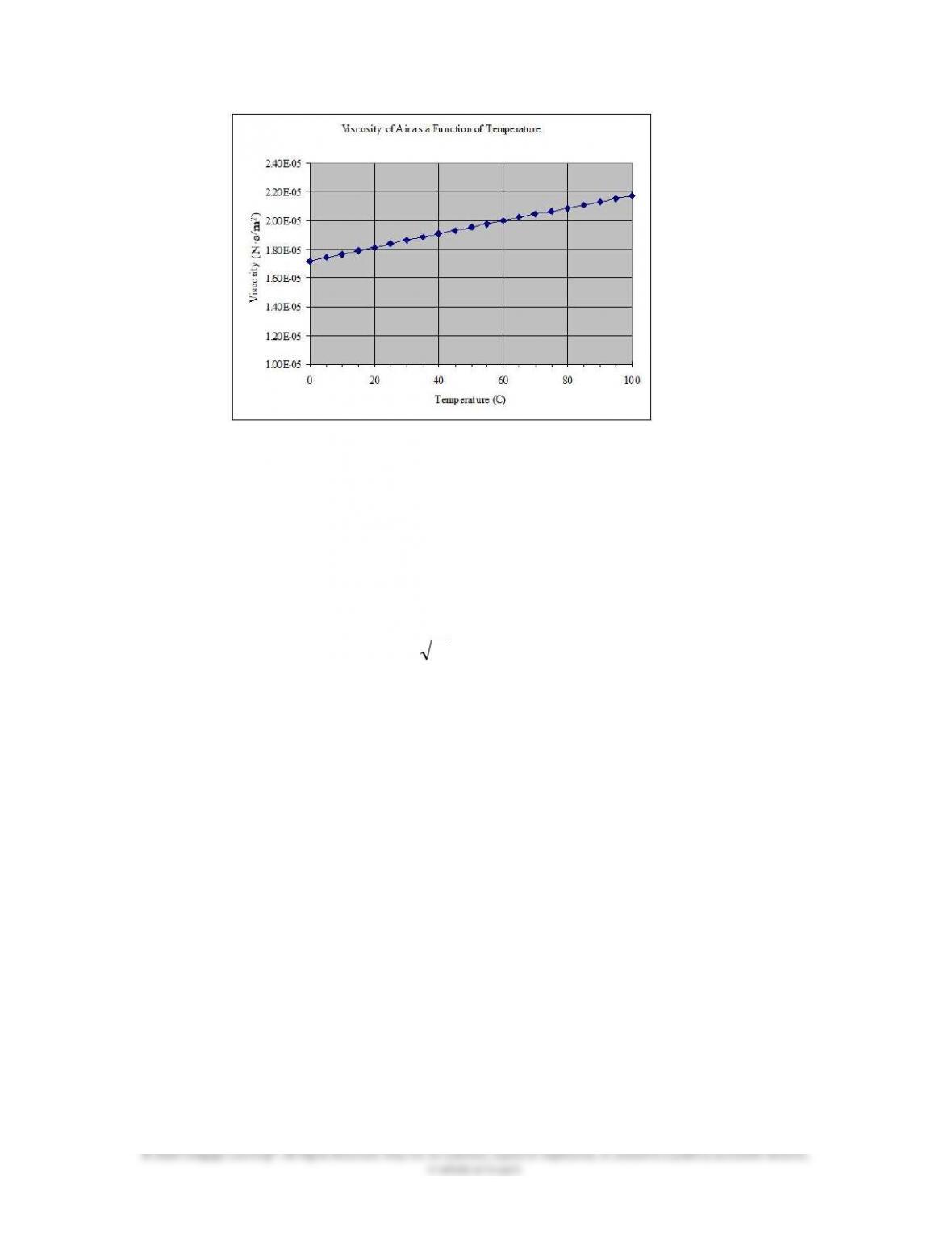
14.18 A person by the name of Sutterland has developed a correlation that can be used
to evaluate the viscosity of air as a function of temperature. It is given by:
T
c
Tc
2
5.0
1
1
where
= viscosity (N·s/m2)
T = temperature (K)
c1 = 1.458×10⁻⁶ ( 2/1
K
s
m
kg
)
c2 = 110.4 K
Create a table that shows the viscosity of air as a function of temperature in the
range of 0 C (273.15 K) to 100 C (373.15 K) in increments of 5 C. Also create
a graph showing the value of viscosity as a function of temperature as shown in
the accompanying spreadsheet.
SOLUTION
Viscosity of Air as a Function of Temperature
Temperature (C) Viscosity (N·s/m2)
0 1.72E-05
10 1.77E-05
20 1.81E-05
30 1.86E-05
40 1.91E-05
50 1.95E-05
60 2.00E-05
70 2.04E-05
80 2.09E-05
90 2.13E-05
100 2.17E-05
194
14.19 In Chapter 11, we explained the concept of windchill factors. We said that the
heat transfer rates from your body to the surrounding increase on a cold, windy
day. Simply stated, you lose more body heat on the cold, windy day than you do
on a calm day. The windchill index accounts for the combined effect of wind
speed and the air temperature. It accounts for the additional body heat loss that
occurs on a cold, windy day. The old windchill values were determined
empirically, and a common correlation used to determine the windchill index was
)33)(1045.10( a
TVVWCI
where
WCI = Wind Chill Index (kcal/m2·h)
V = wind speed (m/s)
Ta = ambient air temperature (C)
and the value 33 is the body surface temperature in degree Celsius.
The more common equivalent wind chill temperature Tequivalent (C)
was given by
33)33)(28.045.1027.5(045.0 5.0 aequivalent TVVT
Note that V is expressed in km/h.
Create a table that shows the windchill temperatures for the range of ambient air
temperature -30 C < Ta < 10 C and wind speed of 20 km/h < V < 80 km/h as
shown in the accompanying spreadsheet.
SOLUTION
A Wind Chill Table
Wind
Ambient Temperature (°C)
speed (km/h)
10 5 0 -5 -10 -15 -20 -25 -30
30 1.0 -6.0 -12.9
-19.9
-26.8
-33.8
-40.7
-47.7
-54.6
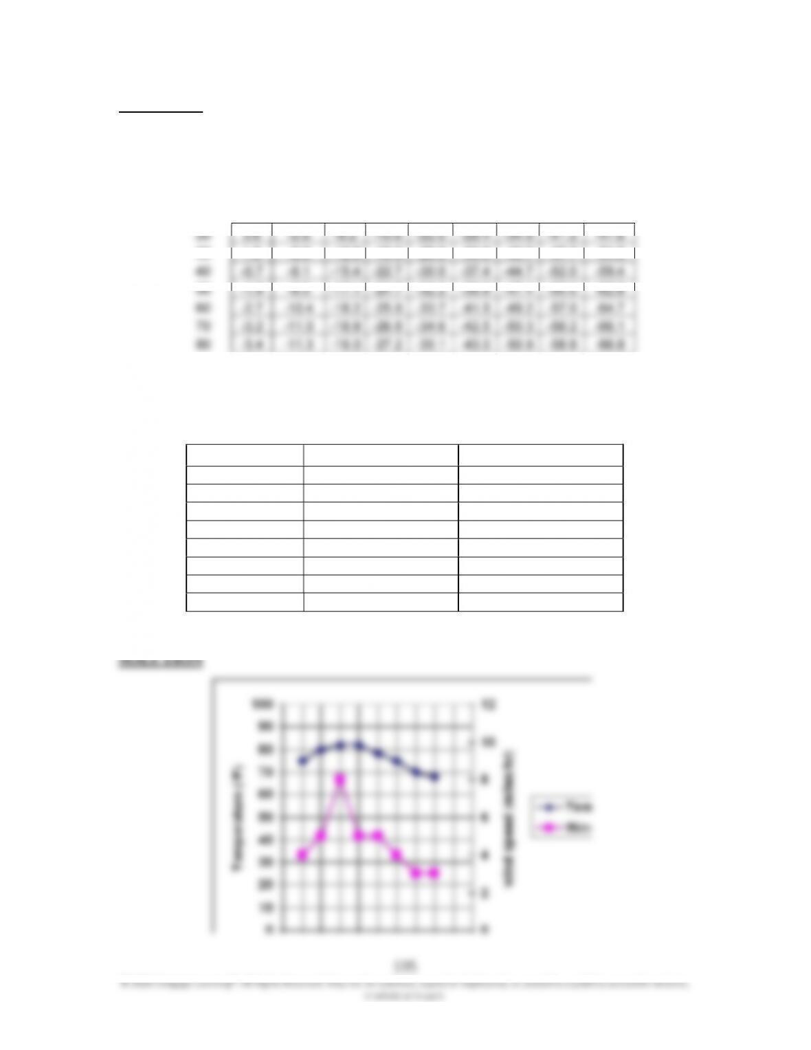
14.21 Use Excel to plot the following data. Use two different y axes. Use a scale of zero
to 100 °F for temperature, and zero to 12 mph for wind speed.
Time (P.M.) Temperature (oF) Wind Speed (mph)
1 75 4
2 80 5
3 82 8
4 82 5
5 78 5
6 75 4
7 70 3
8 68 3
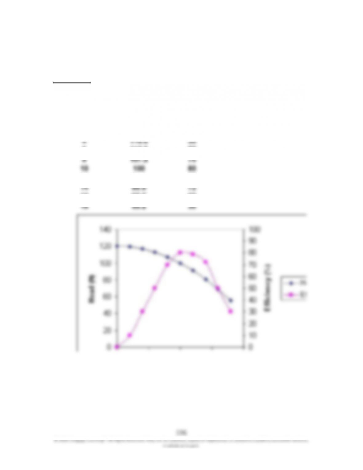
14.22 Use Excel to plot the following data for a pump. Use two different y axes.
Use a scale of zero to 140 ft for the head, and zero to 100 for efficiency.
SOLUTION
Flow Rate
(GPM)
Head of
Pump (ft)
Efficiency (%)
0
120
0
2
119.2
10
4
116.8
30
6
112.8
50
8
107.2
70
10
100
80
12
91.2
79
14
80.8
72
16
68.8
50
18
55.2
30
197
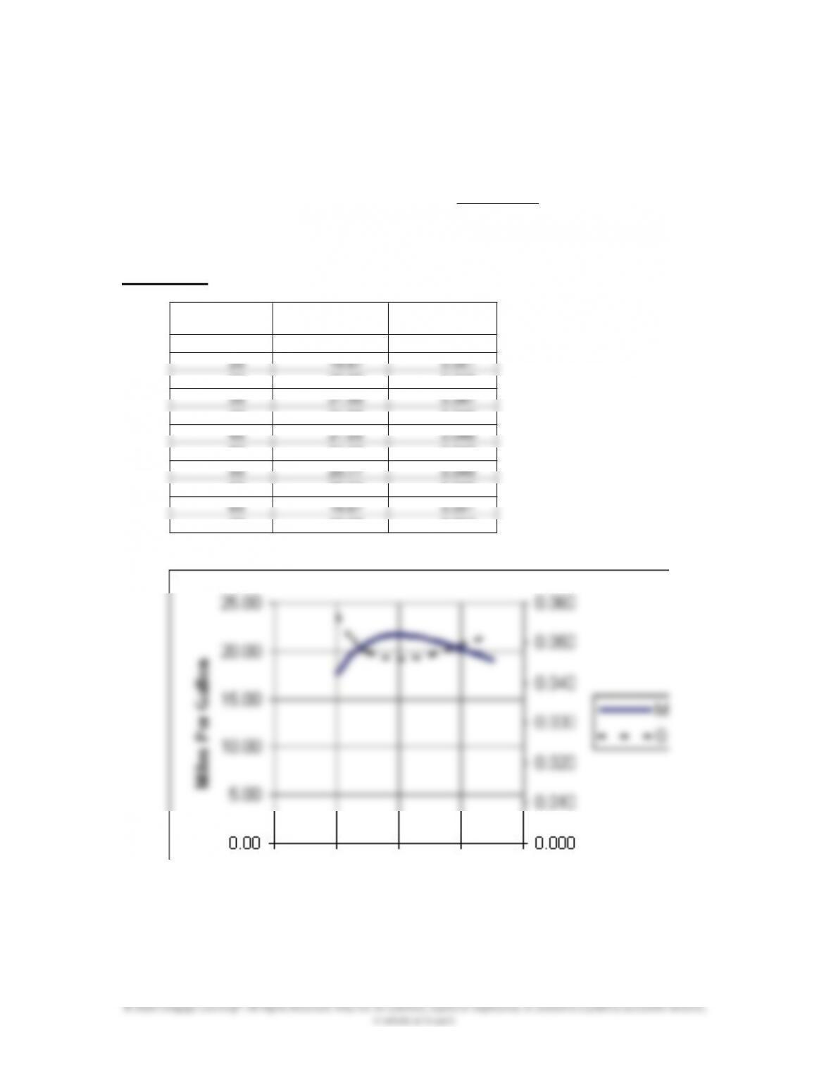
14.23 Use the following empirical relationship to plot the fuel consumption in both
miles per gallon and gallons per mile for a car for which the following
relationship applies. Note: V is the speed of the car in miles per hour and the
given relationship is valid for 30 ≤ V ≤ 70.
SOLUTION
Speed
(mph)
Miles Per
Gallon
Gallons
Per Mile
20 17.66 0.057
30 20.88 0.048
40 21.68 0.046
50 21.23 0.047
60 20.24 0.049
70 19.08 0.052
881
910
1050
Gallon)Per (Miles .
V
V
nConsumptioFuel
198
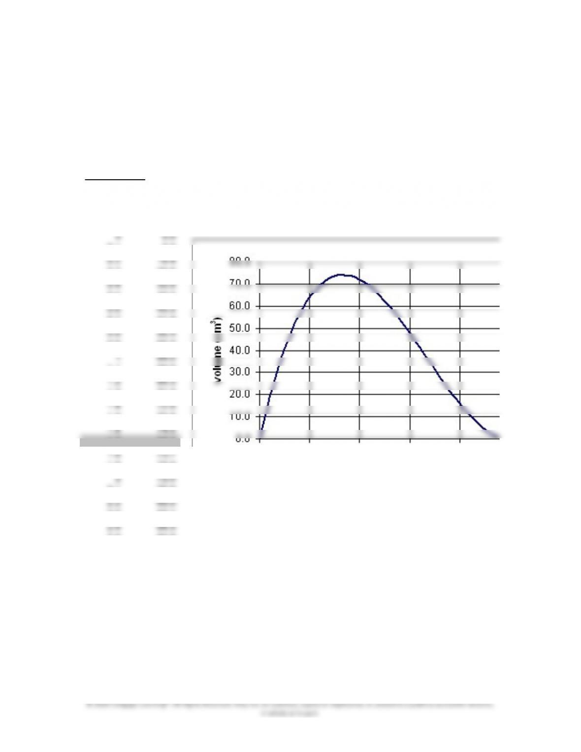
14.24 Starting with a 10 cm × 10 cm sheet of paper, what is the largest volume you can
create by cutting out x cm × x cm from each corner of the sheet and then folding
up the sides. Use Excel to obtain the solution. Hint: the volume created by cutting
out x cm × x cm from each corner of the 10 cm × 10 cm sheet of paper is given
by xxx )210)(210(V
SOLUTION
x
(cm)
(cm
3
)
0.1
9.6
0.3
26.5
0.5
40.5
0.7
51.8
0.9
60.5
1.1
66.9
1.3
71.2
1.5
73.5
1.7
74.1
1.9
73.0
2.1
70.6
2.3
67.1
2.5
62.5
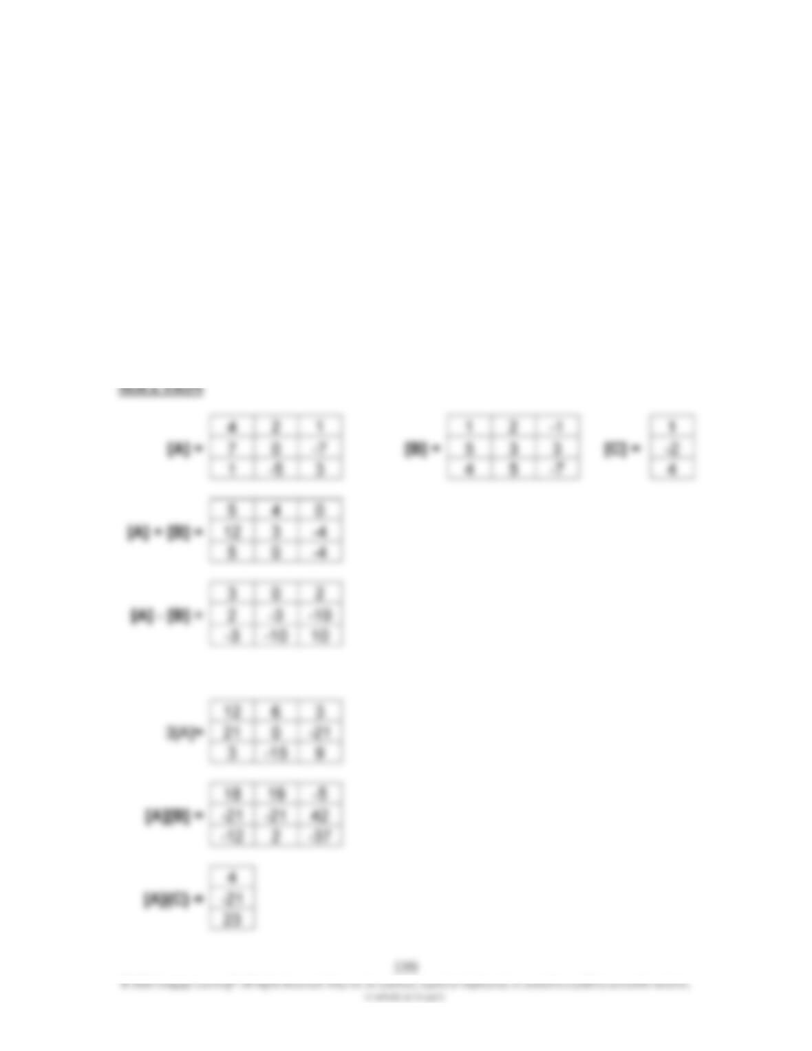
14.25 Given matrices:
351
707
124
A,
754
335
121
B, and
4
2
1
C, perform the following
operations using Excel.
a.
?
BA
b.
?
BA
c.
?3
A
d.
?
BA
e.
?
CA
200
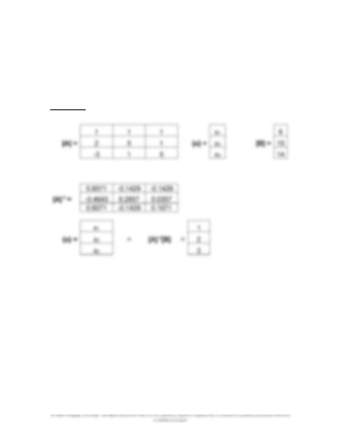
14.26 Solve the following set of equations using Excel.
14
15
6
513
152
111
3
2
1
x
x
x
SOLUTION
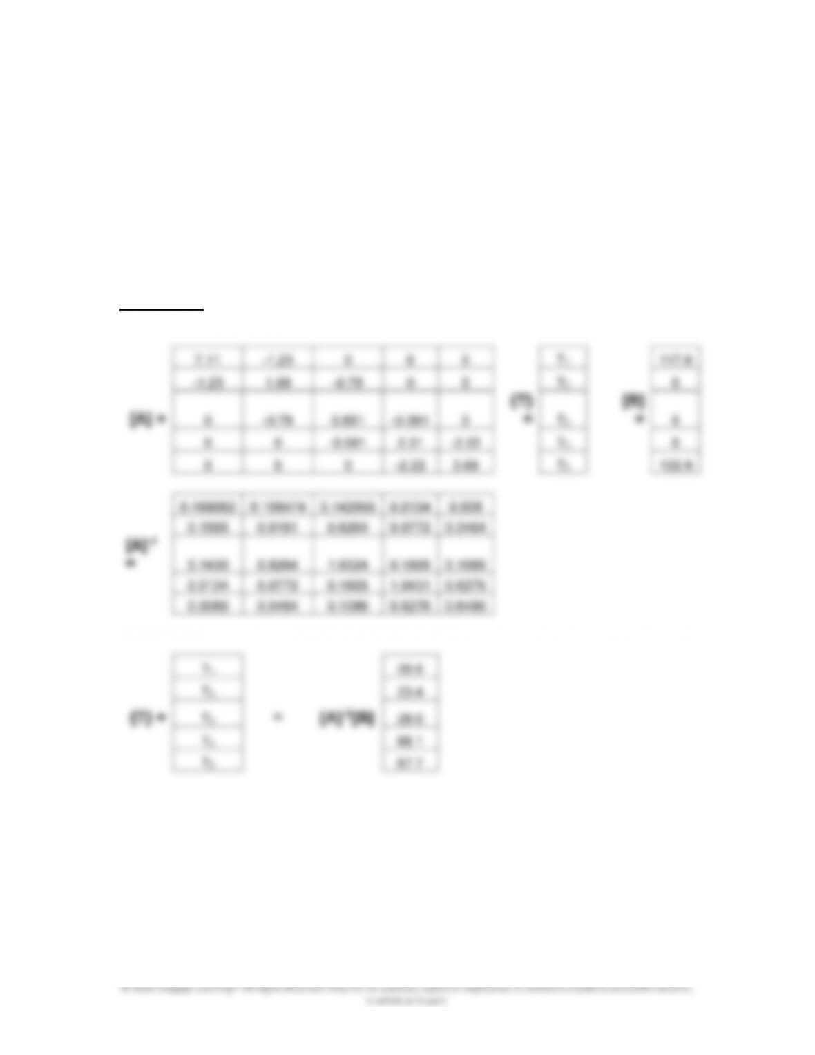
14.27 Solve the following set of equations using Excel.
9.102
0
0
0
6.117
69.322.2000
22.231.2091.000
0091.0851.076.00
0076.099.123.1
00023.111.7
5
4
3
2
1
T
T
T
T
T
SOLUTION
202
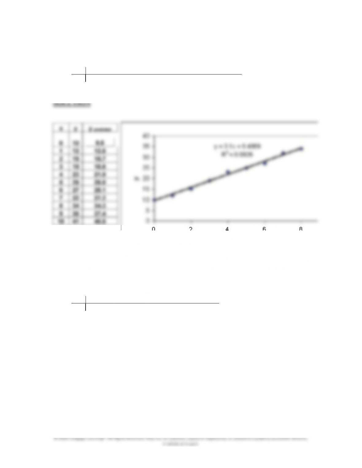
14.28 Find the equation that best fits the following set of data points. Compare the
actual and predicted y values.
x
0
1
2
3
4
5
6
7
8
9
10
y
10
12
15
19
23
25
27
32
34
36
41
14.29 Find the equation that best fits the following set of data points. Compare the
actual and predicted y values.
x
0
1
2
3
4
5
6
7
8
y
5
8
15
32
65
120
203
320
477
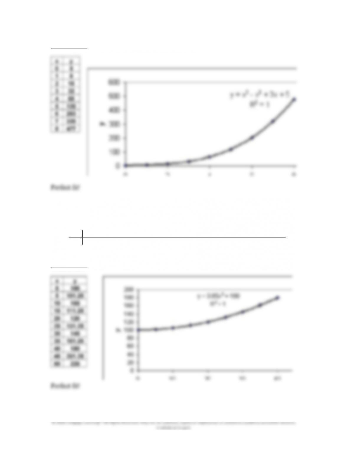
203
SOLUTION
14.30 Find the equation that best fits the following set of data points. Compare the
actual and predicted y values.
x
0
5
10
15
20
2
5
30
35
40
45
50
y
100
101.25
105
111.25
120
131.25
145
161.25
180
201.25
225
SOLUTION