
Problem 14.1
Three alternatives are being evaluated based on six different attributes, all of which are
considered of equal importance. Determine the weight to assign to each attribute.
Problem 14.2
A consultant asked a corporate president to assign importance values from 0 to 100 to
five attributes that will be included in an alternative evaluation. Determine the weight of
each attribute using the president’s importance scores.
Attribute Importance Score
1. Safety40
2. Cost60
3. Impact 70
4. Environmental30
5. Acceptability 50
Problem 14.3
Ten attributes were rank-ordered in terms of increasing importance and were identified as
A, B, C, …, and J. Determine the weight of (a) attribute D, and (b) attribute J.
Problem 14.4
Different types and capacities of crawler hoes are being considered for a pipe-laying
project across the country. Several supervisors who served on similar projects in the past
have identified attributes and their views of relative importance. Determine (a) the
importance scores using a 10 (high) to 0 scale, and (b) the normalized weights using the
weighted rank order approach.
Attribute Comment___________
1 Truck vs. hoe height 90% as important as trenching speed
2 Type of topsoil Only 10% of most important attribute
3 Type of subsoil 30% as important as trenching speed
4 Hoe cycle time Twice as important as type of subsoil
5 Hoe trenching speed Most important attribute
6 Pipe-laying speed 80% as important as hoe cycle time

Problem 14.5
The Athlete’s Shop owner evaluated two proposals for exercise equipment. A present
worth analysis at i = 15% resulted in PWA = $340,000 and PWB = $290,000.
Independently, the lead trainer assigned a relative importance score from 0 to 100 to three
noneconomic attributes, plus the economic attribute.
Attribute Trainer’s Score
Economics 80
Durability 35
Flexibility 30
Maintainability 50
Separately, you have used the four attributes to value rate the proposals on a scale of 0 to
1.0 as shown in the following table.
Value Ratings_______
Attribute Proposal A Proposal B
Economics 1.00 0.90
Durability 0.35 1.00
Flexibility 1.00 0.90
Maintainability 0.25 1.00
Select the better proposal using (a) present worth, and (b) the weighted attribute
method.
Problem 14.6
A public project proposal evaluated at MARR = 6% per year resulted in AW = $5600 per
year and a B/C ratio of 1.7, indicating it is clearly economically justified. The Public
Utility Commission (PUC), which must approve the proposal, uses the weighted attribute
method with four attributes – economic, safety, environmental, and legal – equally
weighted. It is well known that the PUC has never approved a proposal with a weighted
attribute score of at least 100, based on averaged value ratings from each of the three
PUC members. They value rate a proposal using a scale of 0 to 100. The PUC chair
displayed a PowerPoint slide showing the result and rejected the proposal.
Rprop = (economic weight)×(PUC ratingeco) + (safety weight)×(PUC ratingsaf)
+ (environmental weight)×(PUC ratingenv) + (legal weight)×(PUC ratingleg)
= (0.25)×(20) + (0.25)×(40) +(0.25)×(90) +(0.25)×(80)
= 57.5

Since both AW and B/C indicate that approval is warranted, is it possible for the
proposal to be approved by increasing the economic weight determined by the PUC
members?
Problem 14.7
Identify a fundamental reason why all decisions in engineering economics are performed
under risk.
Problem 14.8
For each situation below, determine (a) if the variable is discrete or continuous and (b) if
the information involves certainty or risk.
(1) The first cost of a new front-end loader is $34,000 or $38,000 depending on the size
purchased.
(2) The raises for engineers and technical staff employees will be 3%, or 5%, with half
getting 3% and half getting 5%
(3) Revenue from a new product line is expected to be between $350,000 and $475,000
per year with a larger chance that it is low in the range.
(4) The salvage value for an old machine will be $500 (the asking price) or $0 (it will be
scrapped), depending upon who is selected by the manager to take it.
(5) Profits are expected to be up by anywhere between 25% and 60% this year, with
equal probability for all estimates.
Problem 14.9
Royalty income received by an investor in an oil well will vary according to the price of
oil. Data collected from stripper wells in an established oilfield were used to develop a
probability- royalty relationship. Calculate (a) the expected value of royalties per year,
and (b) the probability that the royalties will be at least $12,600 per year.
Royalties R, $/year 6200 8500 9600 10,300 12,600 15,500
Probability, P(R) 0.10 0.21 0.32 0.24 0.09 0.04
Problem 14.10
The Car Buyer’s Guild surveyed 1000 households to determine the number of operating
vehicles that are owned by residents at the address surveyed. Use the results below to

determine the percentage of households that own (a) 1 or less vehicles; (b) 1 or
2 vehicles, and (c) more than 3 vehicles.
Number of cars, Number of
N Households
0 120
1 560
2 260
3 32
4 22
5 or more 6
Problem 14.11
An engineer was asked to determine whether the average air quality in a volatile chemical
mixing room was within OSHA guidelines. The following air quality readings were
collected: 81, 86, 80, 91, 83, 83, 96, 85, 89.
(a) Determine the arithmetic mean.
(b) Calculate the standard deviation.
(c) Determine the percent of readings that fall within ± 1 standard deviation from the
mean.
(d) Verify your answers using spreadsheet functions.
Problem 14.12
Karen has collected monthly operating expense for the past 3 years for a micro-finishing
department. (a) She wants to know the probability that a month’s expense may be above
$50,000. (b) Provide Karen with the expected value calculated by hand in two forms –
using the number of months and using the probability for each range. Use the midpoints
of each range in preparing the answers.
Expense range, $1000 1-10 10–20 20–30 30–40 40–50 50–60 60–70
Midpoint , $1000 5 15 25 35 45 55 65
Number of months 2 5 8 7 6 5 3

Problem 14.13
A sample of 100 monthly maintenance costs for automated soldering machines was
collected. The costs are clustered into $200 cells with midpoints ranging from $600 to
$2000. The number of times (frequency) each cell value was observed and its probability
are shown below. (a) Find the expected value of the expenses for use in a PW analysis.
(b) Develop the discrete probability distribution of the monthly maintenance costs similar
to Figure 14.1a and indicate the expected value on it.
Cell Midpoint Frequency Probability
600 6 0.06
800 10 0.10
1000 9 0.09
1200 15 0.15
1400 28 0.28
1600 15 0.15
1800 7 0.07
2000 10 0.10
Problem 14.14
A newsstand manager is tracking Y, the number of weekly magazines left on the shelf
when the new edition is delivered. Data collected over a 30-week period are summarized
by a discrete probability distribution. A friend determined that the expected value and
standard deviation of these results are E(Y) = 7.08 and sY = 3.23, respectively. Plot the
distribution and indicate the expected value and one standard deviation on either side of
it.
Copies, Y 3 7 10 12
P(Y) 1/3 1/4 1/3 1/12
Problem 14.15
When using Monte Carlo sampling to obtain random numbers from the probability
distributions of varying parameters, what is a fundamental assumption that must be
made?
Problem 14.16
Use the RAND()*100 spreadsheet function to generate 100 values from a uniform
distribution with the range of 0 to 100. Then use other spreadsheet functions to calculate
(a) the average and compare the sample value to 50, and (b) the standard deviation and

compare the sample value to 28.87. These two values are correct for a continuous
uniform distribution with limits of 0 and 100.
Problem 14.17
(a) Explain the meaning of a sample standard deviation.
(b) Use the Excel© help utility to determine the formula used by the STDEV function.
Problem 14.18
Use the Excel© help utility to determine what the following functions are designed to do:
(a) VLOOKUP, and (b) RANDBETWEEN.
Problem 14.19
Carl, a colleague in Europe working for the same company that you do, estimated cash
flow after taxes (CFAT) for a project he is working on.
Year CFAT, $
0 -35,000
1–10 5,500
The PW value at the current MARR of 8% per year is:
PW = -35,000 + 5500(P/A,8%,10) = $1905
Because of the changing economic scene, Carl believes the MARR will vary over a
relatively narrow range, as will the CFAT. He is willing to accept the other estimates as
certain. Use the following probability distribution assumptions for MARR and CFAT to
perform a simulation. Take a sample of 30 or more simulation trials. Is the project
economically justified using decision making under certainty? Under risk?
MARR Discrete uniform distribution over the range 7% to 10%
CFAT Continuous uniform distribution over the range $4000 to
$7000 for each year
Problem 14.20
Janice is a process engineer for Upland Chemicals. Yesterday, she was handed the
following information about a piece of air quality sampling equipment that she earlier
requested be purchased for her department. The request was denied by the Corporate
Finance Manager based on the large negative PW value that she calculated.
P = $-150,000
GI = $50,000 per year
E = 10% of P or $-15,000 per year
n = 10 years
S = 20% of P or $30,000
PW = $-21,811
Janice was quite aggravated when she determined the interest rate used in the analysis
was 25%, well above the published corporate MARR of 10% to justify required product
or environmental quality equipment. In a meeting with her, she shared some of her own
estimates with you about first cost and expected life. Using the following estimates and
distribution assumptions, perform a simulation for Janice that may help her in an effort to
obtain approval of the equipment’s purchase.
Accepted as certain: GI = $50,000 per year
E = 10% of P
S = 20% of P
Varying: P Continuous uniform distribution over the range
$-100,000 to $-150,000
n Discrete uniform distribution over the range 8 to 15 years
MARR Discrete uniform distribution; values from 10% through
15% have a 15% chance each; values from 16% to 25%
have a 1% chance each
Problem 14.21
All of the following are excellent attribute identification approaches except:
a. Employing small group discussions
b. Using the same attributes that competing entities use
c. Getting input from experts with relevant experience
d. Surveying the stakeholders
Problem 14.22
If attributes of first cost, safety, and environmental concerns had scores of 100, 75, and
50, respectively, the weight for environmental concerns will be closest to:
a. 0.44

b. 0.33
c. 0.22
d. 0.11
Problem 14.23
Alternative locations for a new drinking water treatment plant are being evaluated using
four attributes identified as A, B, C, and D with weights of 0.4, 0.3, 0.2, and 0.1,
respectively. If the value rating scale is from 1 to 10, the evaluation measure of the
weighted attribute method for ratings of 3, 7, 2, 10 for attributes A, B ,C, and D,
respectively, is closest to:
a. 3.3
b. 3.9
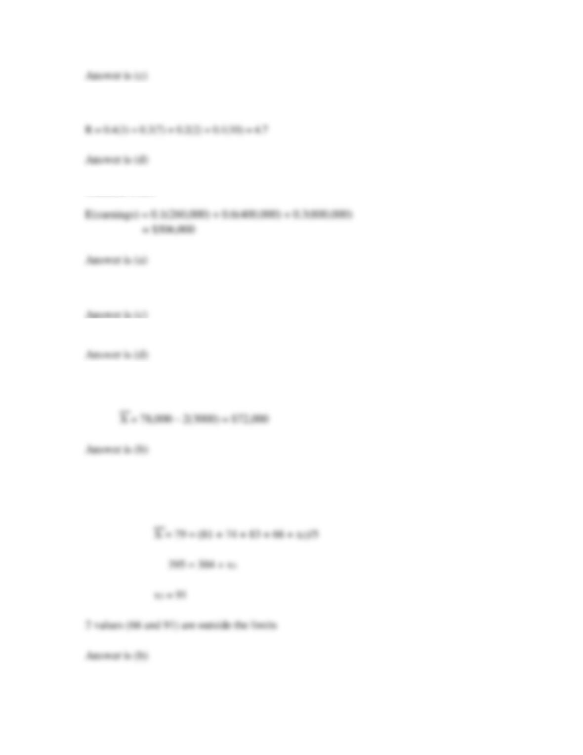
c. 4.1
d. 4.7
Problem 14.24
The president of Bullnose Shoes estimated the chances of different levels of earnings for
this calendar year . They are:
Earnings Chance
$260,000 1 in 10
$400,000 6 in 10
$800,000 3 in 10
The expected value of the earnings is closest to:
a. (a) $506,000
b. (b) $493,000
c. (c) $461,000
d. (d) $402,000
Problem 14.25
A prime difference between a discrete and continuous random variable is:
a. a discrete variable can only take on integer values.
b. a continuous variable cannot have negative values.
c. a discrete variable can only assume isolated values.
d. in the highest and lowest values that they can assume.
Problem 14.26
A fundamental assumption made when obtaining a random sample from the probability
distribution of a variable is that:
a. the distribution must be discrete or continuous uniform.
b. once set, the sample size cannot be increased.
c. the sample size must be large enough to estimate the actual value within
±5%.
d. no other variable affects the one being sampled .
Problem 14.27
You were informed that the highest salary of engineers in your department was $78,000
per year and that this was two standard deviations above the average. If you discover that
the standard deviation is $3000, the average salary is closest to:
a. $66,000
b. $72,000
c. $75,000
d. $81,000
Problem 14.28
The historic average and standard deviation of the percentage moisture content MC of a
product is E(MC) = 78.5% and sMC = 10.5%, respectively. The results of a sample of size
5 taken over the last 5 hours included the following data: 81, 74, 83, 66, X = 79. If the
guideline is to maintain the product’s moisture within 1 standard deviation of the historic
average, the number of sample values outside these limits is:
a. 3
b. 2
c. 1
d. none
Solution 14.1
Solution 14.2
Solution 14.3
Solution 14.4
(a) Score by attribute with 10 for most important
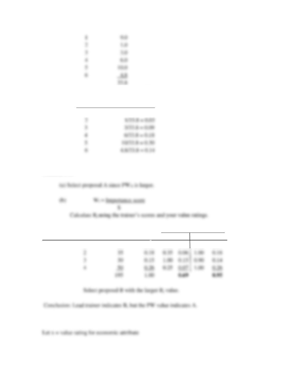
(b) Normalized weights, Wi = Score/33.8
Attribute Wi______
1 9/33.8 = 0.27
Solution 14.5
Attribute Importance Rj________________
i Score Wi Value A Value B__
1 80 0.41 1.00 0.41 0.90 0.37
Solution 14.6
Solution 14.7
Solution 14.8
(1) Discrete and Certainty
Solution 14.9
Solution 14.10
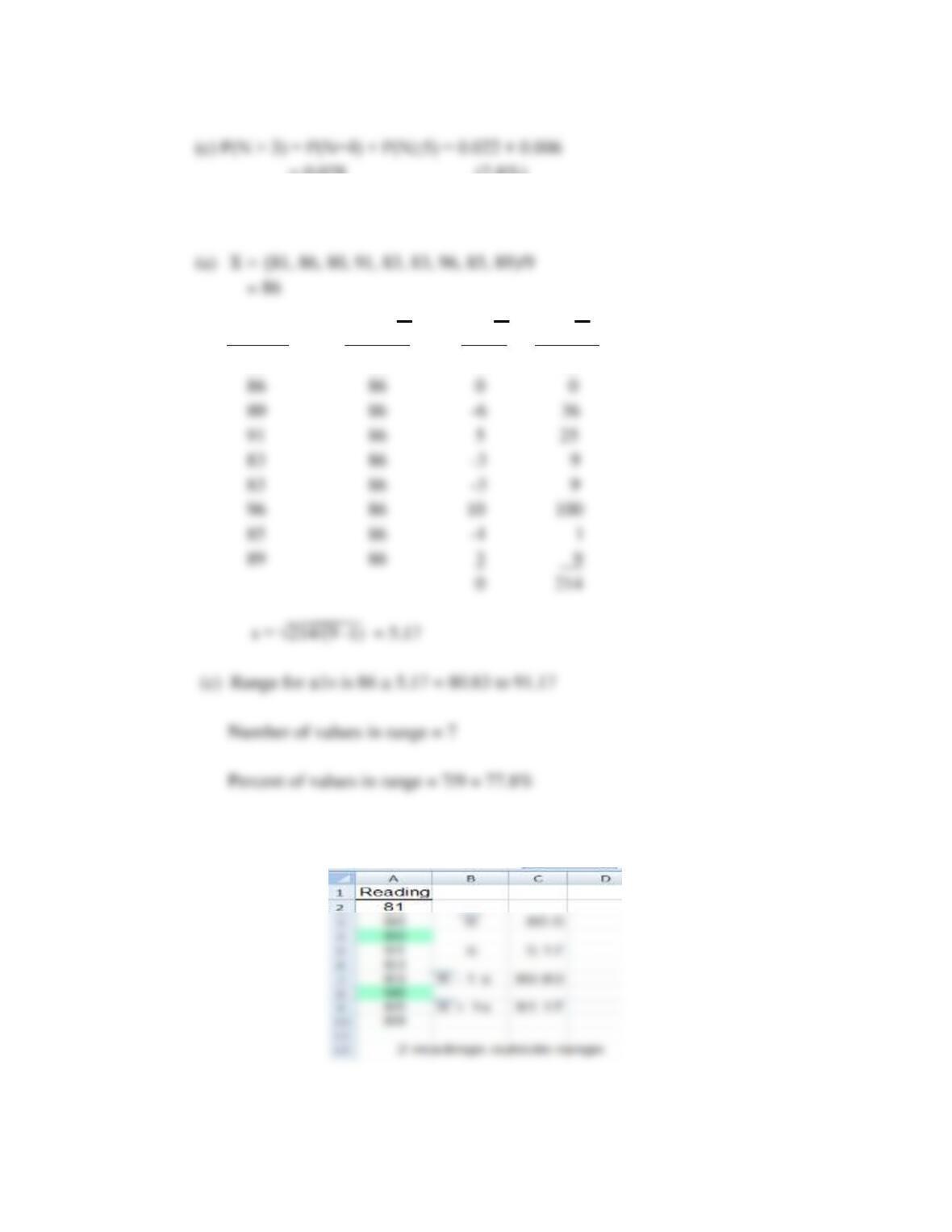
Determine the probability values for N.
N 0 1 2 3 4_ ≥5_
= 0.028 (2.8%)
Solution 14.11
(b) Reading Mean, X Xi – X (Xi – X)2
81 86 -5 25
(d) Spreadsheet confirmation using AVERAGE and STDEV functions.
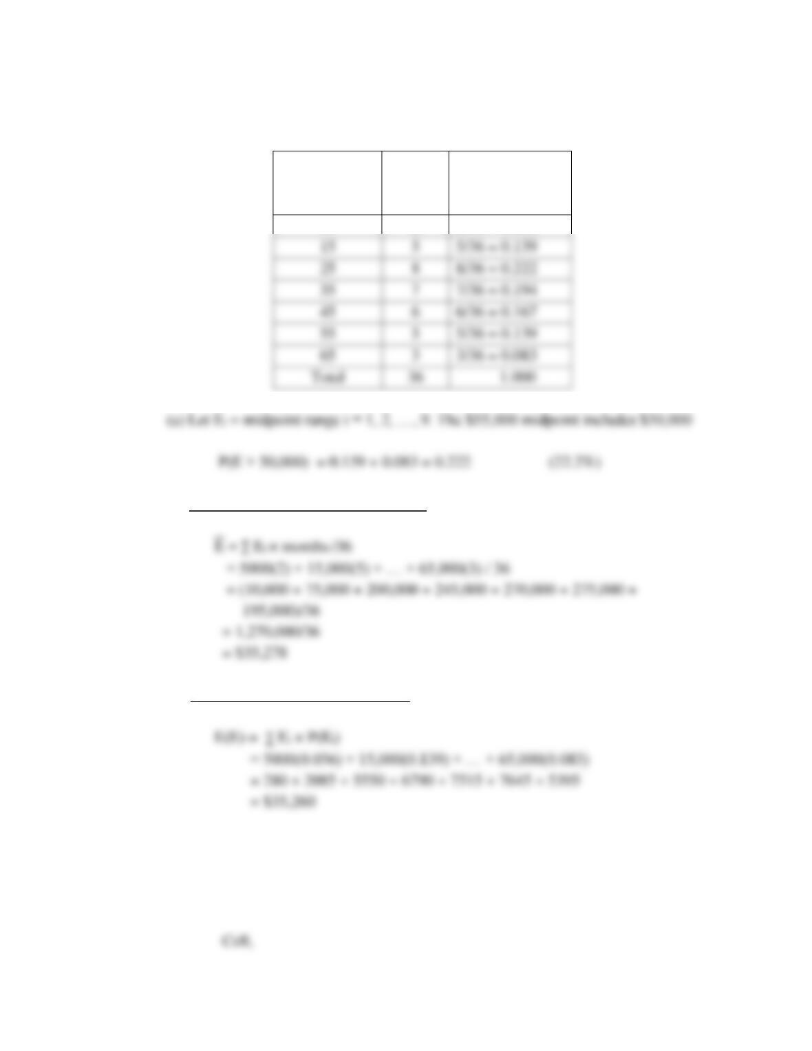
Solution 14.12
Expense range
midpoint,
$1000
Number
of
months
Probability
5
2
2/36 = 0.056
(b) Average using number of month data:
Expected value using probabilities:
Solution 14.13
(a) Use Equation [14.5] to find E(X).
5
5/36 = 0.139
6
6/36 = 0.167
5
5/36 = 0.139
3
3/36 = 0.083
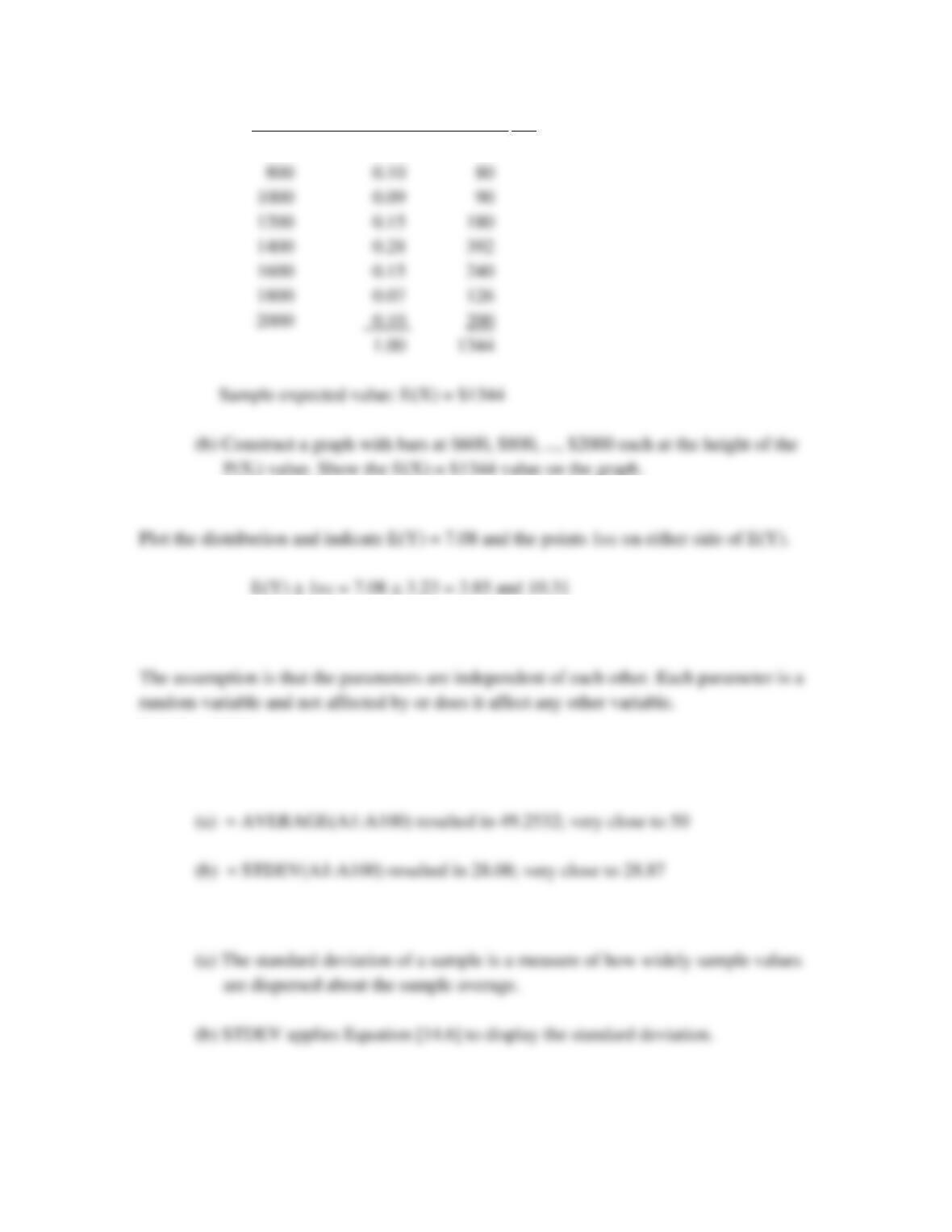
Xi, $ P(Xi) Xi × P(Xi), $
600 0.06 36
Solution 14.14
Solution 14.15
Solution 14.16
As an example, a sample of 100 values generated the following results:
Solution 14.17
Solution 14.18
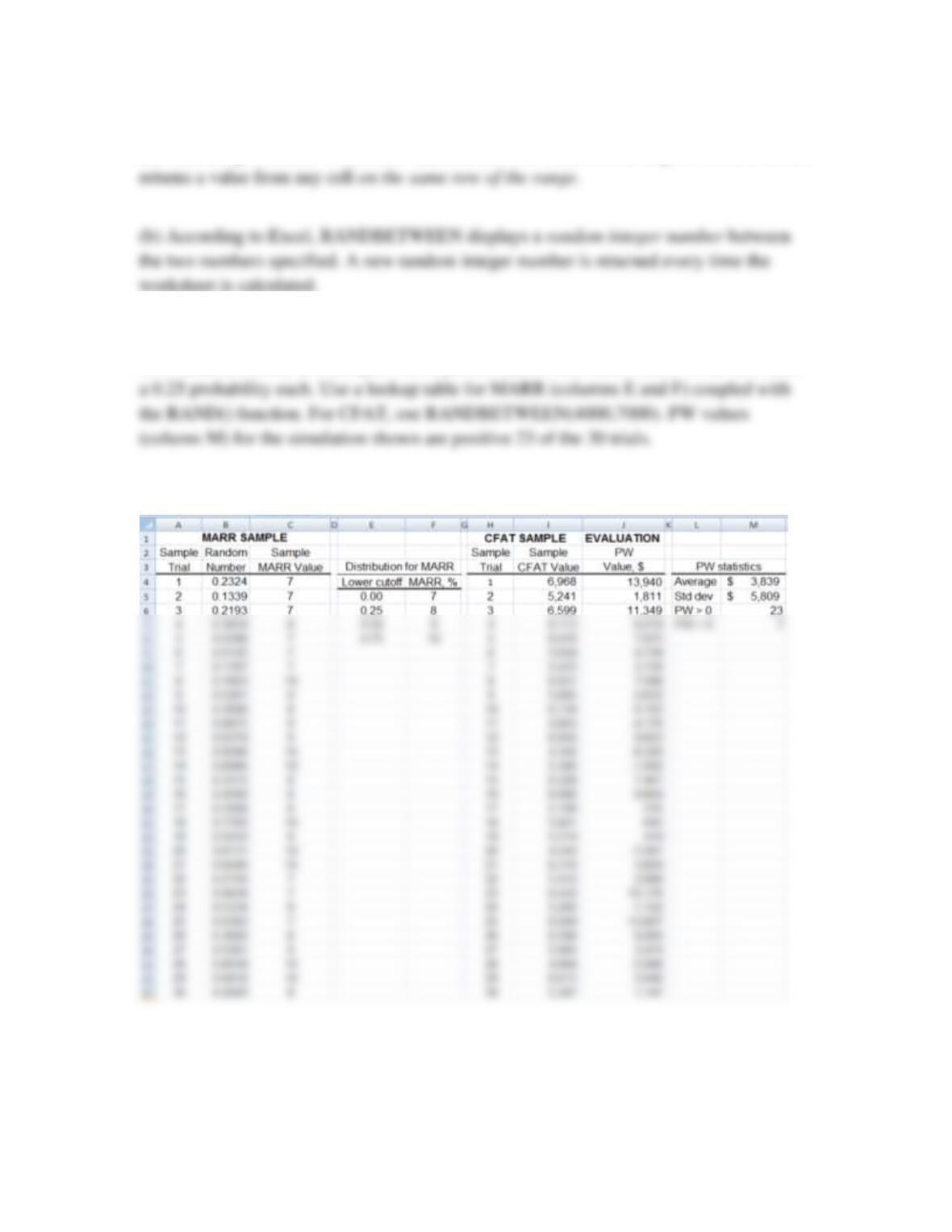
(a) According to Excel, VLOOKUP searches the first column of a range of cells, and then
worksheet is calculated.
Solution 14.19
A simulation similar to Example 14.6 is performed. MARR varies from 7% to 10% with
Conclusion: The project appears economically viable under both certainty and risk.
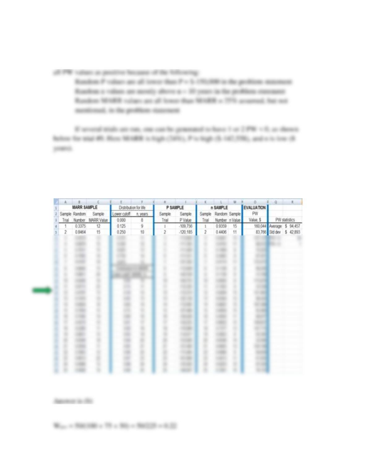
Solution 14.20
A simulation patterned after that of Example 14.6 is shown below. Most trails will show
Conclusion: The simulation runs show that, for the varying estimates that Janice has
presented, the equipment is virtually always justified with PW > 0.
Solution 14.21
Solution 14.22
Solution 14.23
Solution 14.24
Solution 14.25
Solution 14.26
Solution 14.27
Solution 14.28
Reading #5 is missing