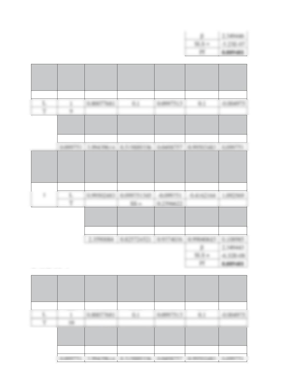
14-33
T=9 H=? L=1
Random
variable
Mean
Value
Mean for
equivalent
Normal
Standard
Deviation
Standard
Deviation of
Equivalent
Normal
Coefficient of
Variation Py
H 3.15 3.08685171 0.4725 0.4698741 0.15 1.136277
Vy
Lognormal
Distribution,
fx
Lognormal
Cumulative, Fx )-1(Fx(x*)) Px
N Vx
N
0.149166 0.84668262 0.529726894 0.0745832 3.11495529 0.469874
Iteration Random
variable
Mean for
equivalent
normal
Standard
deviation for
equivalent
normal
Partial
derivative
Directional
cosine
New
design
point
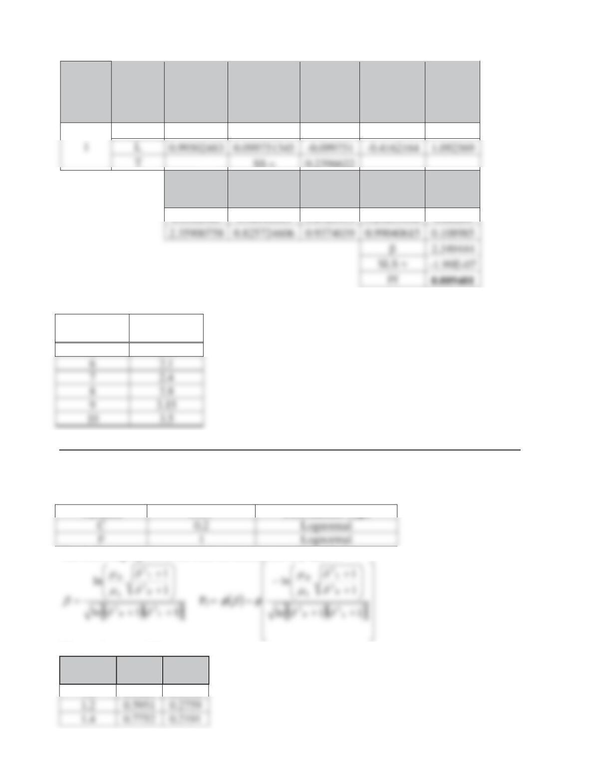
H 3.11495529 0.469874097 -0.217917 -0.9092656 4.118732
Lognormal
Distribution,
fx
Lognormal
Cumulative, Fx )-1(Fx(x*)) Px
N Vx
N
0.11255159 0.969410088 1.8721927 2.96850112 0.614376
T=10 H=? L=1
Random
variable
Mean
Value
Mean for
equivalent
Normal
Standard
Deviation
Standard
Deviation of
Equivalent
Normal
Coefficient of
Variation Py
H 3.5 3.44316654 0.525 0.5220823 0.15 1.241638
Vy
Lognormal
Distribution,
fx
Lognormal
Cumulative, Fx )-1(Fx(x*)) Px
N Vx
N
0.149166 0.76201436 0.529726894 0.0745832 3.46106143 0.522082
14-34
Iteration Random
variable
Mean for
equivalent
normal
Standard
deviation for
equivalent
normal
Partial
derivative
Directional
cosine
New
design
point
H 3.46106143 0.52208233 -0.217917 -0.9092656 4.576369
Lognormal
Distribution,
fx
Lognormal
Cumulative, Fx )-1(Fx(x*)) Px
N Vx
N
0.1012963 0.96941013 1.8721933 3.29833446 0.68264
Summary of results:
T H
5 1.75
Problem 14-13.
The performance function can be expressed as:
Z = C/F –1
Where C and F are random variables. The following information is given:
Variable COV Distribution Type
The following equations are used for calculation of E and Pf
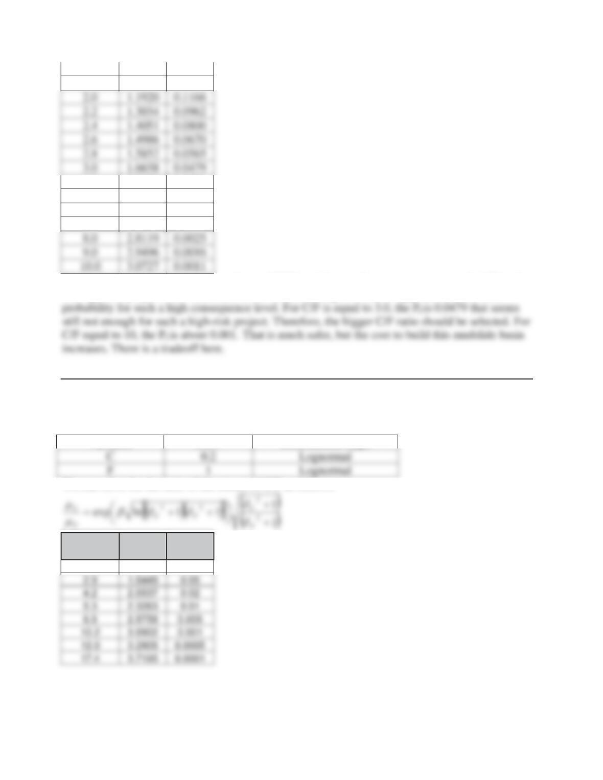
The results are as follows:
Mean Ratio
of C/F ȕ Pf
1.0 0.3821 0.3512
14-35
1.6 0.9313 0.1759
1.8 1.0689 0.1426
4.0 2.0020 0.0226
5.0 2.2627 0.0118
6.0 2.4758 0.0066
7.0 2.6559 0.0040
The highway with average traffic volume of 5000 vehicles per day at an average speed of 50 mph
is a high-risk project. The mean ratio of C/F should be high in order to approach a low failure
Problem 14-14.
The performance function can be expresses as:
Z = C/F – 1
Where C and F are random variables. The following information is given:
Variable COV Distribution Type
We can solve for the ratio of the means of C/F as follows:
Mean Ratio
of C/F ȕ Pf
2.2 1.2816 0.1
14-36
Problem 14-15.
The parameters of the distributions are:
I P L E A
mean 100 20 30000 1
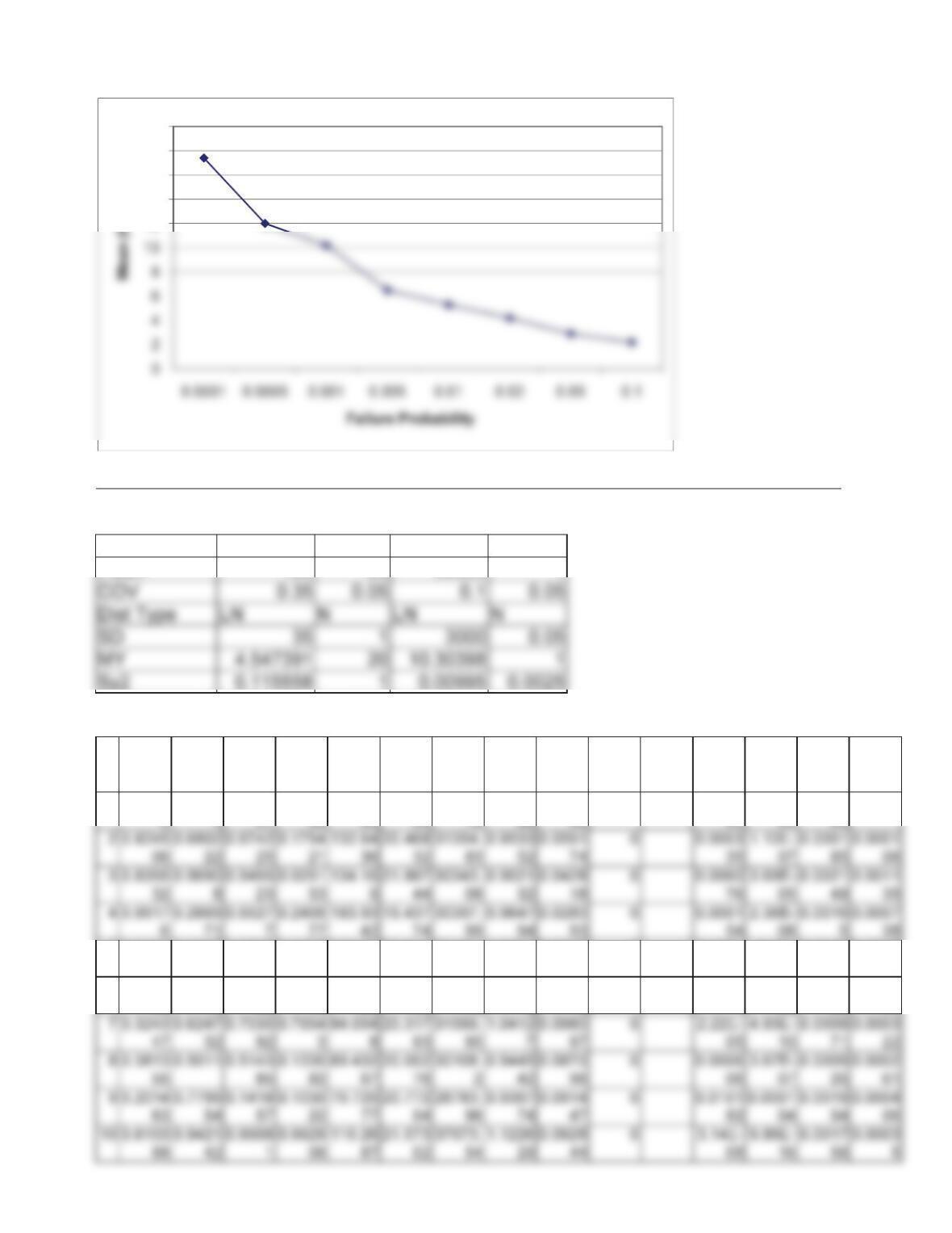
The following table shows the results of 10 simulation cycles, in which P was used as the control
variable in the CE method:
i u1 u2 u3 u4 P L E A z=PL/(
AE)-
0.1
PF
Direct
COV(
Pf
Direct)
Pfi for
CE
Pfi^2
for CE
Mean(
Pf CE)
COV(
Pf CE)
1 0.0173
3
0.4135
4
0.5846
37
0.7474
38
46.032
05
19.781
55
30494.
49
1.0333
22
0.1211
02
0 3.6E–
05
1.3E-
09
3.6E-
05
na
5 0.5430
63
0.6337
08
0.8538
46
0.9037
55
103.78
54
20.341
69
33159.
22
1.0651
62
0.0902
27
0 2.28E-
06
5.2E-
12
0.0013
21
0.0005
32
6 0.0845
53
0.6098
14
0.1958
88
0.9867
16
51.872
25
20.278
84
27430.
79
1.1108
9
0.1154
8
0 0.0001
7
2.89E-
08
0.0011
29
0.0004
04
12
14
16
18
20
14-37
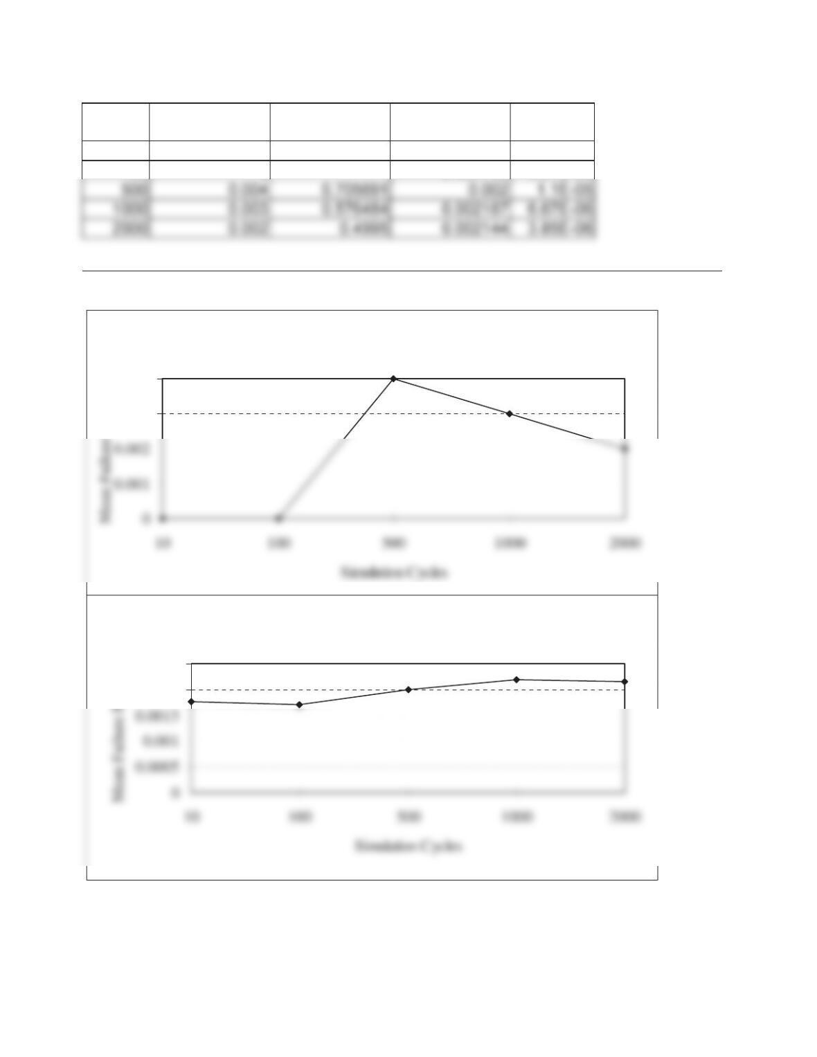
The results for different numbers of cycles are shown in the following table:
N Direct, Mean Pf Direct, COV(Pf) CE, Mean Pf CE,
COV(Pf)
10 0 0.001758 0.00035
100 0 0.001708 5.57E-05
Problem 14-16.
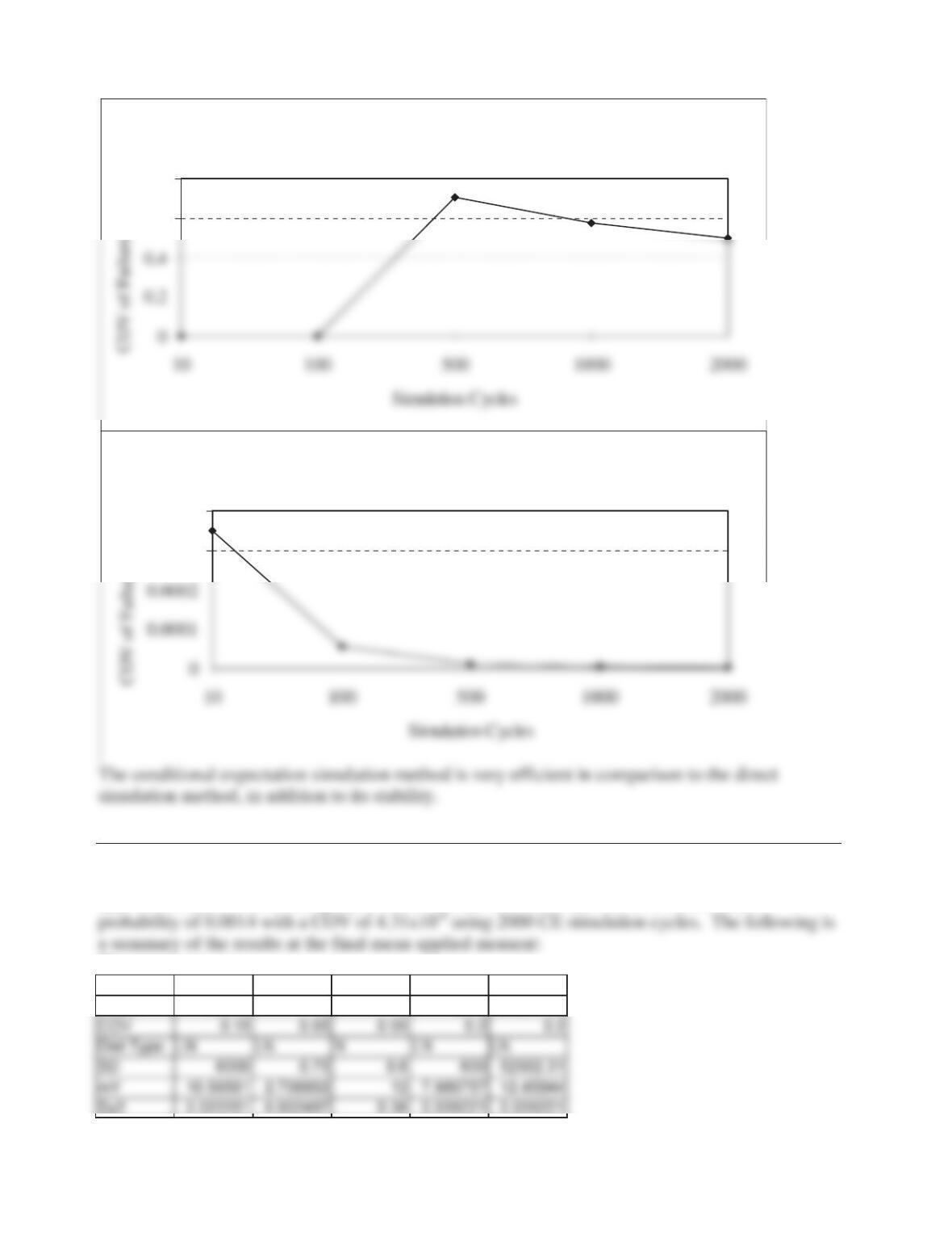
The results for this problem are show in Problem 14-15. The following figures present the results:
Direct Simulation
0.003
0.004
t
Conditional Expectation Simulation
0.002
0.0025
t
14-38
Problem 14-17.
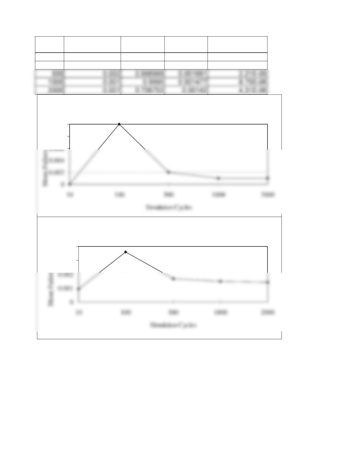
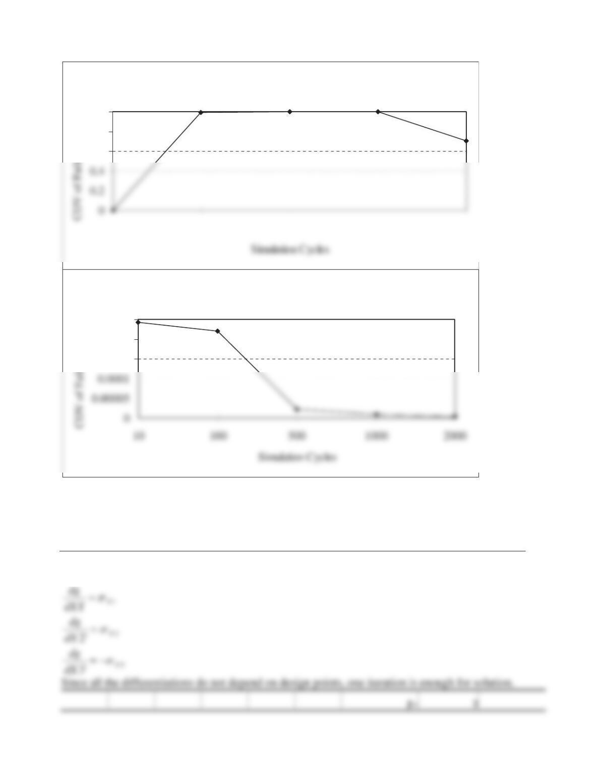
A simulation program was developed to allow the incremental change of the mean strength of the
applied moment. The resulting mean value is 262,512 lb-in that produces a main failure
The parameters are
F=As*fy d b fc’ M
mean 40000 15 12 3000 262511.5
The results are
Direct Simulation
0.6
0.8
t
Conditional Expectation Simulation
0.0003
0.0004
t
14-39
N Direct, Mean Pf Direct,
COV(Pf)
CE, Mean Pf CE, COV(Pf)
10 0 0.000928 0.000242
100 0.01 0.994987 0.003593 0.000221
Direct Simulation
0.008
0.01
t
Conditional Expectation Simulation
0.003
0.004
t
14-40
14.7. Reliability-Based Design
Problem 14-18.
321
X
X
X
g
Direct Simulation
0.6
0.8
1
t
Conditional Expectation Simulation
0.00015
0.0002
0.00025
t
14-41
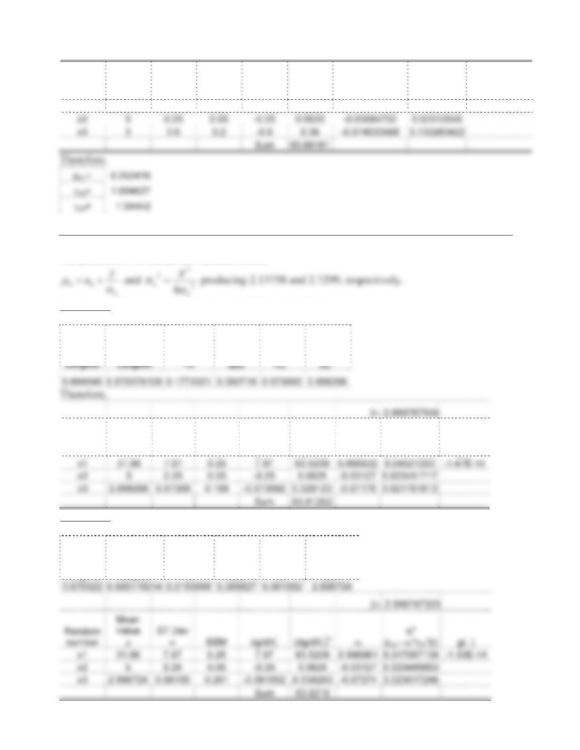
Random
number
Mean
Value
P
ST Dev
VCOV dg/dXi
‘ (dg/dXi
‘)2Di
xi*
(Pxi –Di*Vxi*E)g(..)
x1 32.31329 8.078324 0.25 8.078324 65.25931 0.996778548 8.15639553 -3.81768E-07
Problem 14-19.
The parameters Dn and Pn are calculated from
Iteration 1: (These equations produce 2.13758 and 2.7299, respectively.)
The equivalent normal for the third variable is
fx(x*)
for Type-
1
Fx(x*)
for Type-1
)Fx(x*))
N Pxi
N
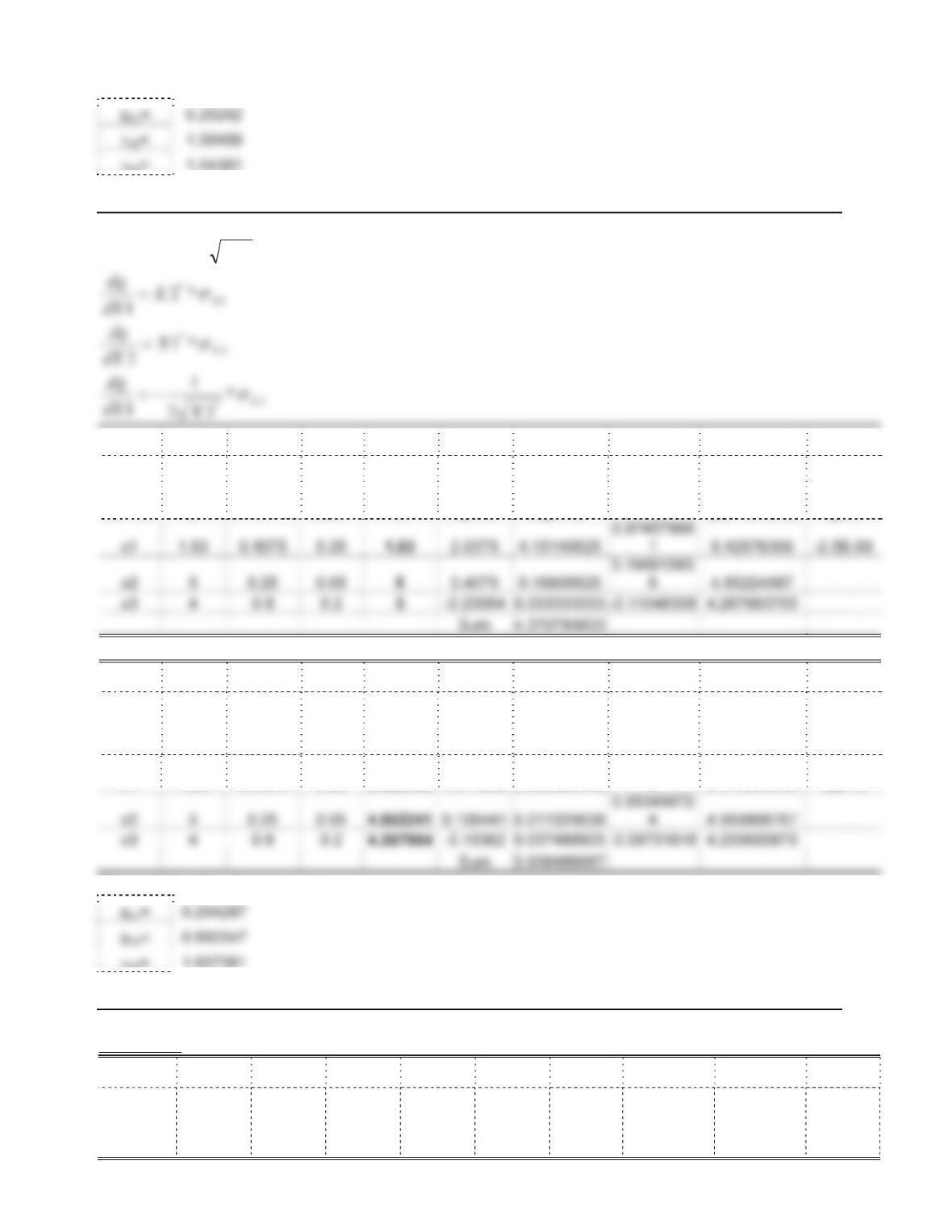
Random
number
Mean
Value
P
ST Dev
VCOV dg/dXi
‘ (dg/dXi
‘)2Di
xi*
(Pxi –Di*Vxi*E) g(..)
Iteration 2:
The equivalent normal for the third variable is
fx(x*)
for Type-
1
Largest
Fx(x*)
for Type-1
Largest
)Fx(x*))
=z I(z) Vxi
N Pxi
N
The partial safety factors are
14-42
Problem 14-20.
32*1
XXXg
1
E
3.032263679
Random
number
Mean
Value
P
ST Dev
VCOV
Design
Point
xi dg/dXi
‘ (dg/dXi
‘)2Di
xi* =
(Pxi –Di*Vxi*E) g(..)
2
E
3.00053758
Random
number
Mean
Value
P
ST Dev
VCOV
Design
Point
xi dg/dXi
‘ (dg/dXi
‘)2Di
xi* =
(Pxi –Di*Vxi*E)g(..)
x1 1.63 0.4075 0.25 0.425763 1.977288 3.909668446
0.99381459
5 0.414843949 -2E-10
The partial safety factors are
Problem 14-21.
Iteration 1:
Random
number
Mean
Value
P
ST Dev
VCOV
Mean
Value
P
y
ST Dev
V
y
Design
point
x*
fx(x*)
for
lognormal
Fx(x*)
for
lognormal
)Fx(x*))
=z
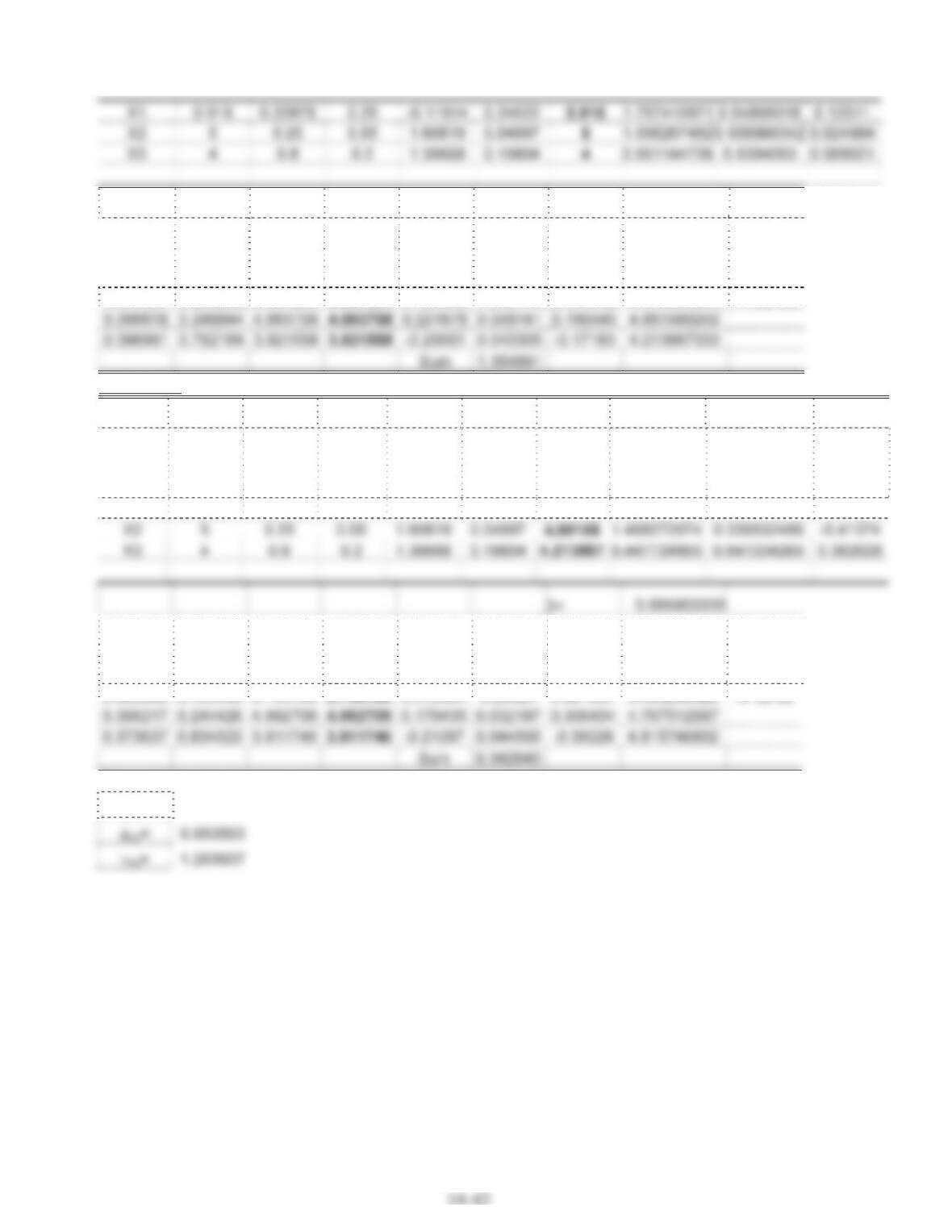
E 2.147423146
I(z) Vxi
N Pxi
N
Design
Point
xi dg/dXi
‘ (dg/dXi
‘)2Di
xi* =
(Pxi –Di*Vxi*E) g(..)
0.39593 0.225292 0.887264 0.887264 1.125053 1.265745 0.966542 0.419653854 -7.6E-08
Iteration 2:
Random
number
Mean
Value
P
ST Dev
VCOV
Mean
Value
P
y
ST Dev
V
y
Design
point
x*
fx(x*)
for
lognormal
Fx(x*)
for lognormal
)Fx(x*))
=z
X1 0.915 0.22875 0.25 -0.11914 0.24622 0.419654 0.03769715 0.001172306 -3.04266
I(z) Vxi
N Pxi
N
Design
Point
xi dg/dXi
‘ (dg/dXi
‘)2Di
xi* =
(Pxi –Di*Vxi*E) g(..)
The partial safety factors are
IX1=0.503059