14-1
CHAPTER 14. RELIABILITY ANALYSIS OF COMPONENTS
CHAPTER 14. RELIABILITY ANALYSIS OF COMPONENTS ……………………………………………1
14.1. Introduction …………………………………………………………………………………………………………….1
14.2. Time to Failure ………………………………………………………………………………………………………..1
14.3. Reliability of Components …………………………………………………………………………………………1
14.4. to 14.6. Reliability Assessments Methods (FORM, ASM, and Simulation) ……………………..1
14.7. Reliability-Based Design …………………………………………………………………………………………40
The following table provides a summary of the problems with their appropriate sections:
Section Problems
14.1 to 14.3 None
14.4 and 14.6 1 to 17
14.7 18 to 21
14.1. Introduction
None
14.2. Time to Failure
None
14.3. Reliability of Components
None
14.4. to 14.6. Reliability Assessments Methods (FORM, ASM, and
Simulation)
Problem 14-1.
a. First-order Reliability Analysis
Using first-order reliability analysis based on first-order Taylor series, the following can be
obtained:
a. Advanced Second-moment Reliability Analysis
14-2
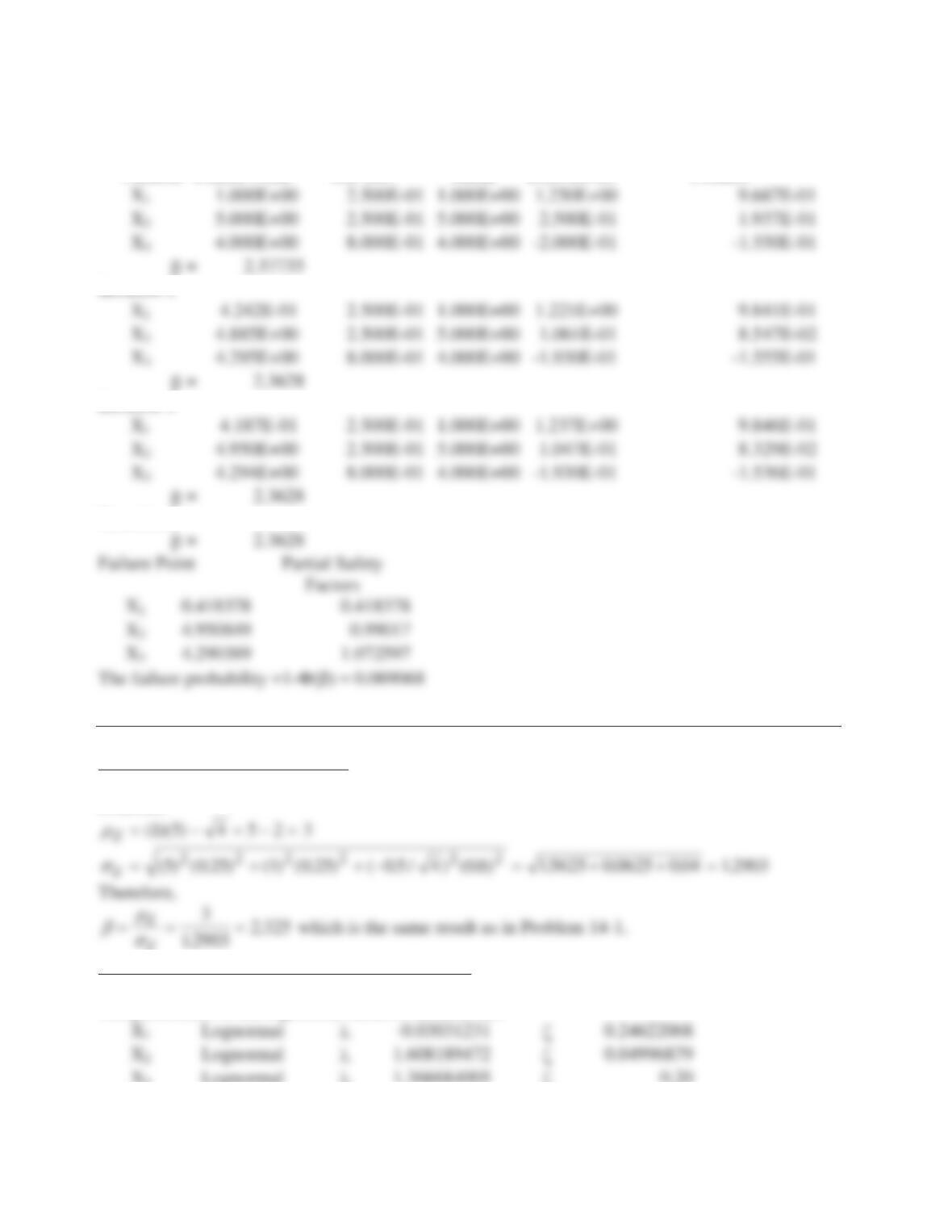
Using advanced second-moment reliability analysis, the following table can be constructed:
Iteration 1
Random Assumed Eq. Normal Eq. Normal Partial Direction
Variable Failure Point Std. Dev Mean Derivatives Cosines
Iteration 2
Iteration 3
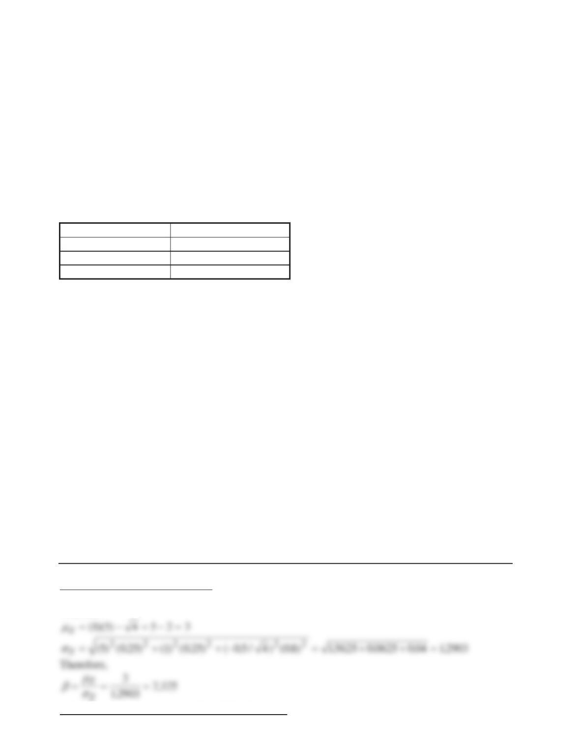
Therefore,
Problem 14-2.
a. First-order Reliability Analysis
Using first-order reliability analysis based on first-order Taylor series, the following can be
obtained:
Z
a. Advanced Second-moment Reliability Analysis
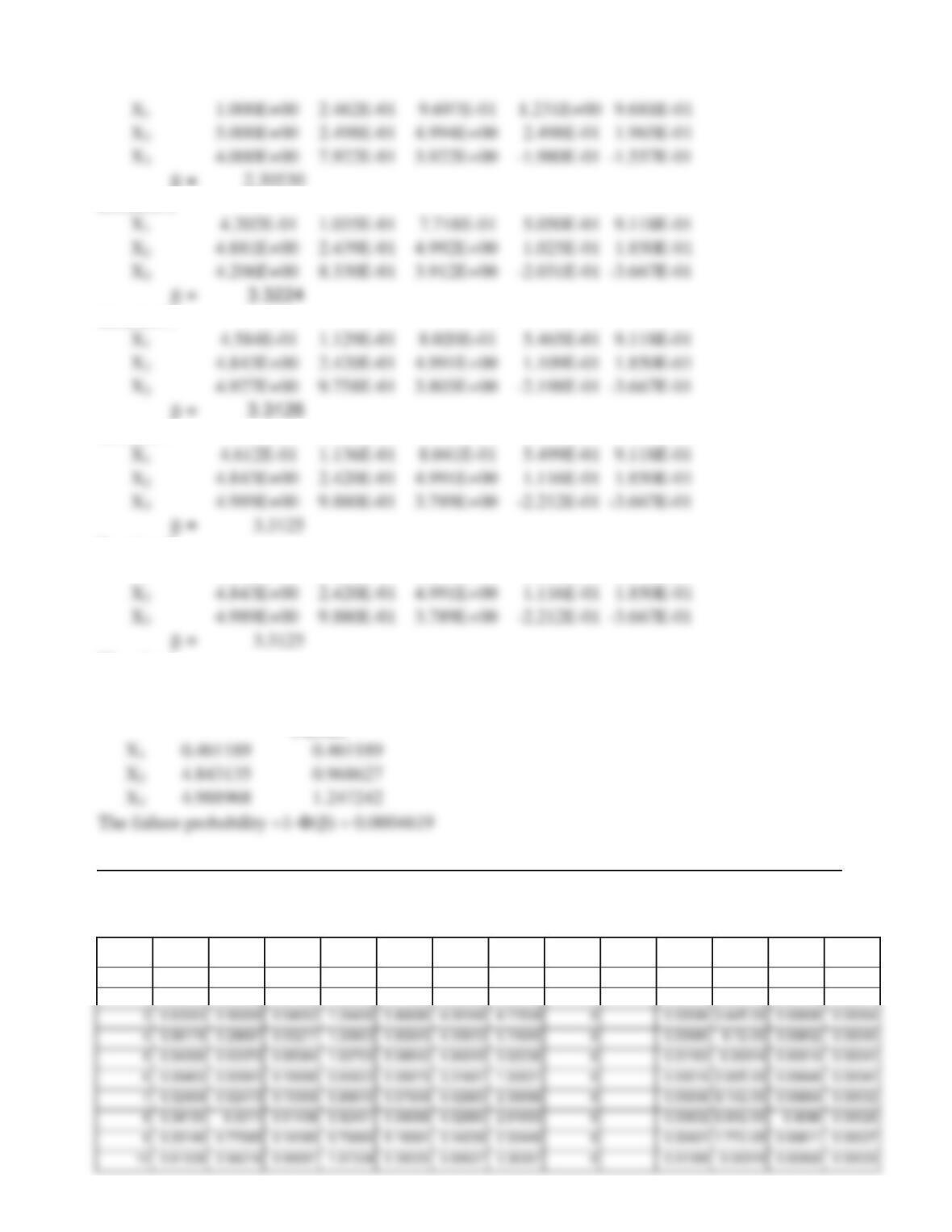
Using advanced second-moment reliability analysis, the following table can be constructed:
The parameters of the lognormal random variables are
X3 Lognormal O 1.366684005 ] 0.20
Iteration 1
Random Assumed Eq. Normal Eq. Normal Partial Direction
Variable Failure Point Std. Dev Mean Derivatives Cosines
14-3
E = 2.30530
Iteration 2
Iteration 3
Iteration 4
Iteration 5
X1 4.612E-01 1.136E-01 8.041E-01 5.500E-01 9.118E-01
Therefore,
E = 3.3125
Failure Point Partial Safety
Factors
Problem 14-3.
The following table shows the results of 10 simulation cycles, in which X1 was used as the control
variable in the CE method:
i u1 u2 u3 x1 x2 x3 z=x1x2-
sqrt(x3)
PF
Direct
COV(Pf
Direct)
Pfi for
CE
Pfi^2 for
CE
Mean(Pf
CE)
COV(Pf
CE)
1 0.01733 0.41354 0.58463 0.47192 4.94538 4.17101 0.29154 0 0.00943 8.9E-05 0.00943 na
2 0.82450 0.68022 0.67422 1.23316 5.11708 4.36128 4.22185 0 0.00895 8.02E-05 0.00919 0.00017
14-4
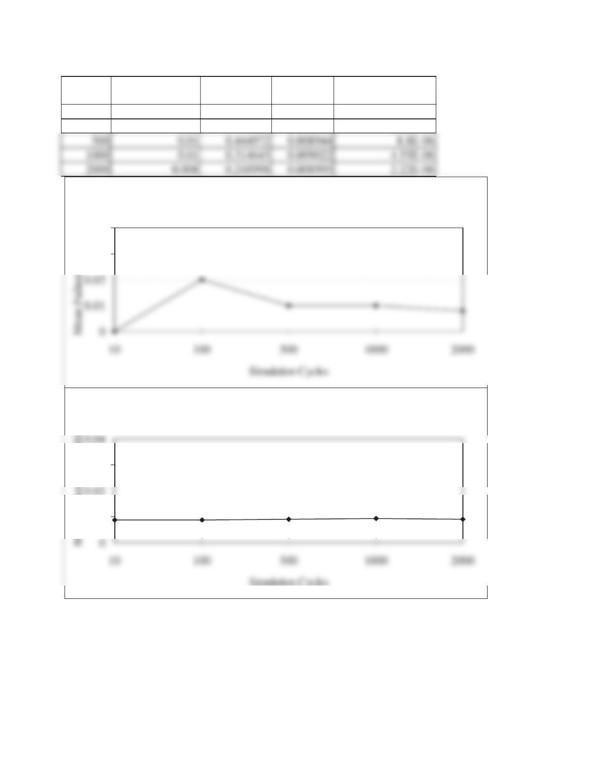
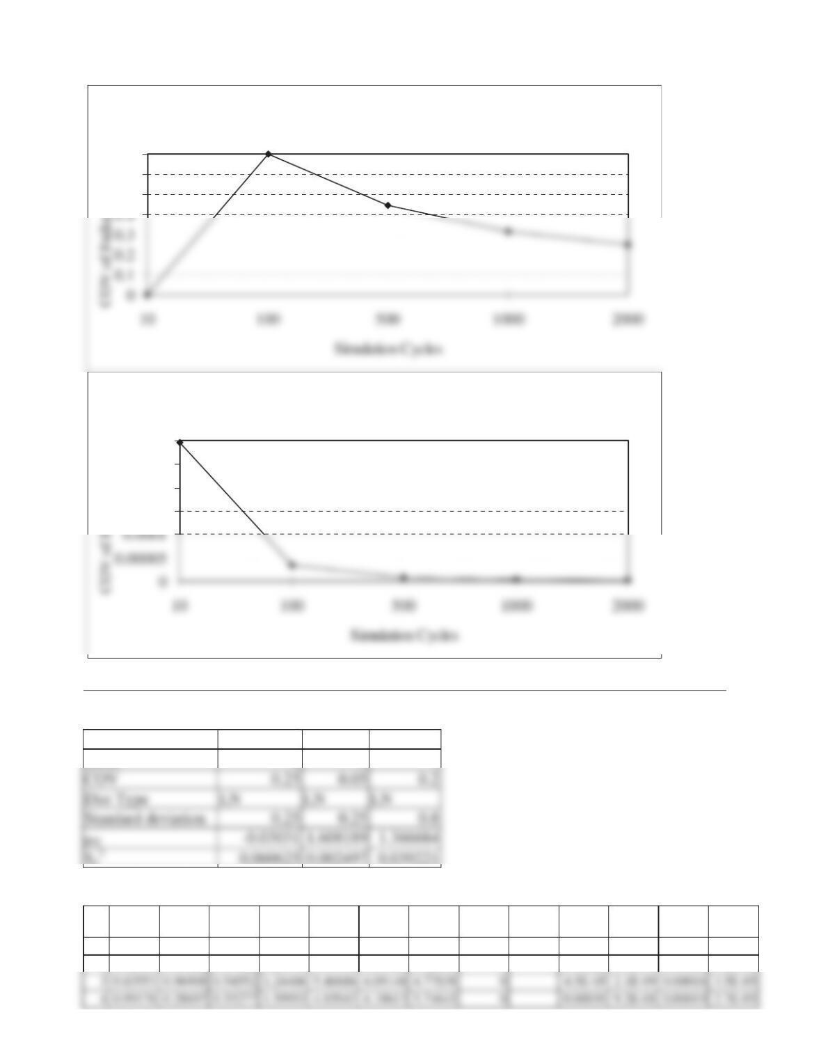
The results for different numbers of cycles are shown in the following table and figures:
N Direct, Mean Pf Direct,
COV(Pf)
CE, Mean
Pf
CE, COV(Pf)
10 0 0.008689 0.000296
100 0.02 0.7 0.008503 3.52E-05
Direct Simulation
0.03
0.04
t
Conditional Expectation Simulation
0.01
0.03
14-5
Problem 14-4.
The parameters of the lognormal distributions are given by
X1 X2 X3
mean 1 5 4
y
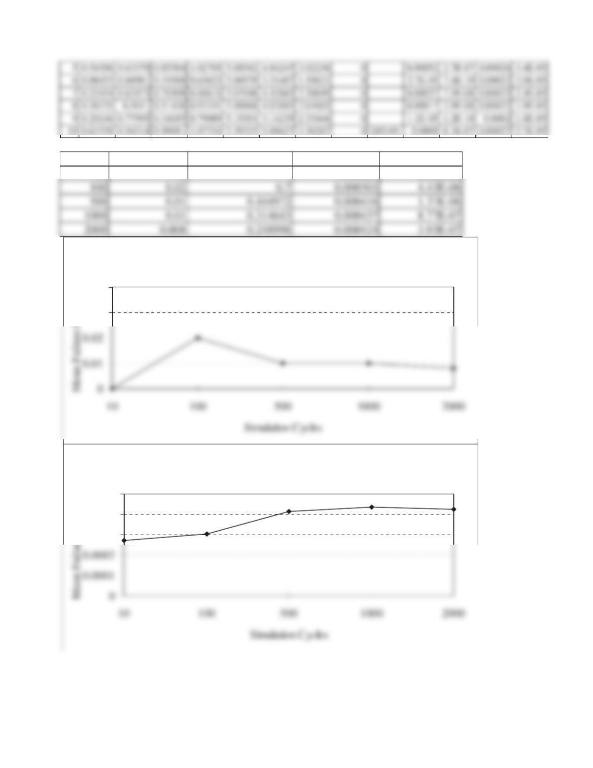
The following table shows the results of 10 simulation cycles, in which X1 was used as the control
variable in the CE method:
i u1 u2 u3 x1 x2 x3 z=x1x2-
sqrt(x3)
PF
Direct
COV(Pf
Direct)
Pfi for
CE
Pfi^2
for CE
Mean(P
f CE)
COV(Pf
CE)
1 0.01733 0.41354 0.58463 0.57671 4.93954 4.09194 0.82586 0 0.00023 5.3E-08 0.00023 na
2 0.82450 0.68022 0.67422 1.23316 5.11708 4.36128 4.22185 0 0.00022 4.8E-08 0.00022 4.2E-06
Direct Simulation
0.5
0.6
0.7
t
Conditional Expectation Simulation
0.00015
0.0002
0.00025
0.0003
t
14-6
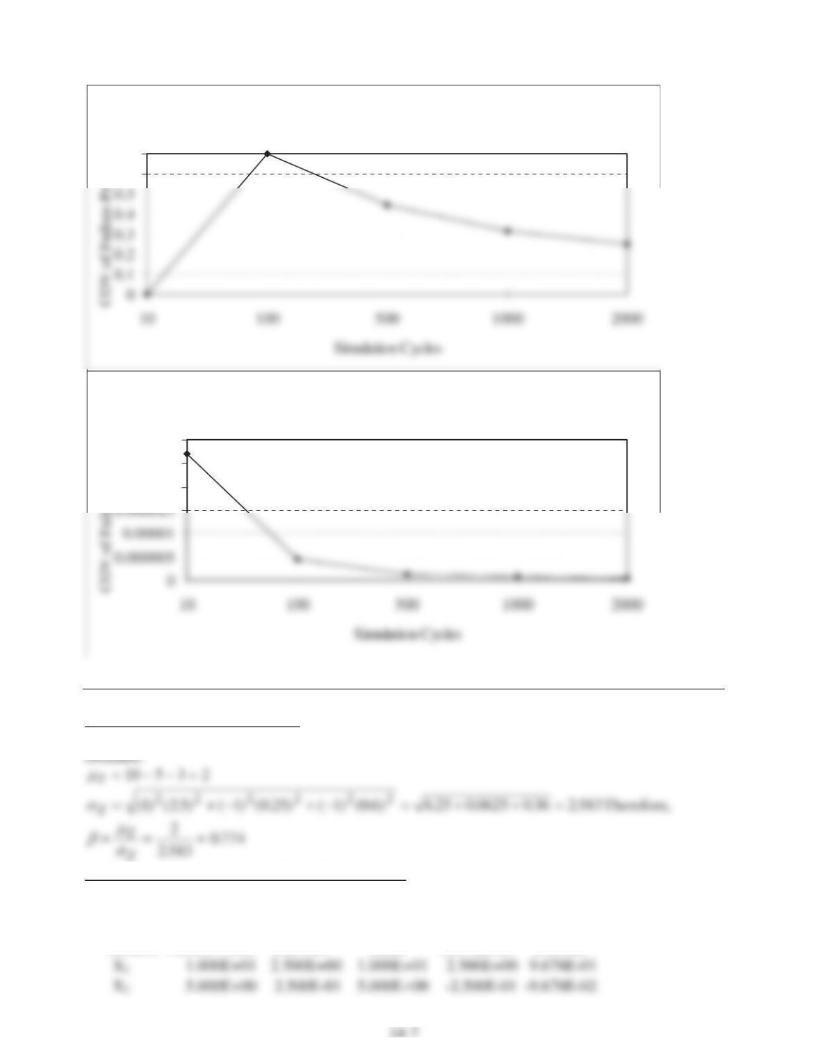
The results for different numbers of cycles are shown in the following table and figures:
N Direct, Mean Pf Direct, COV(Pf) CE, Mean Pf CE, COV(Pf)
10 0 0.00027 2.69E-05
Direct Simulation
0.03
0.04
t
Conditional Expectation Simulation
0.0003
0.0004
0.0005
t
Problem 14-5.
a. First-order Reliability Analysis
Using first-order reliability analysis based on first-order Taylor series, the following can be
a. Advanced Second-moment Reliability Analysis
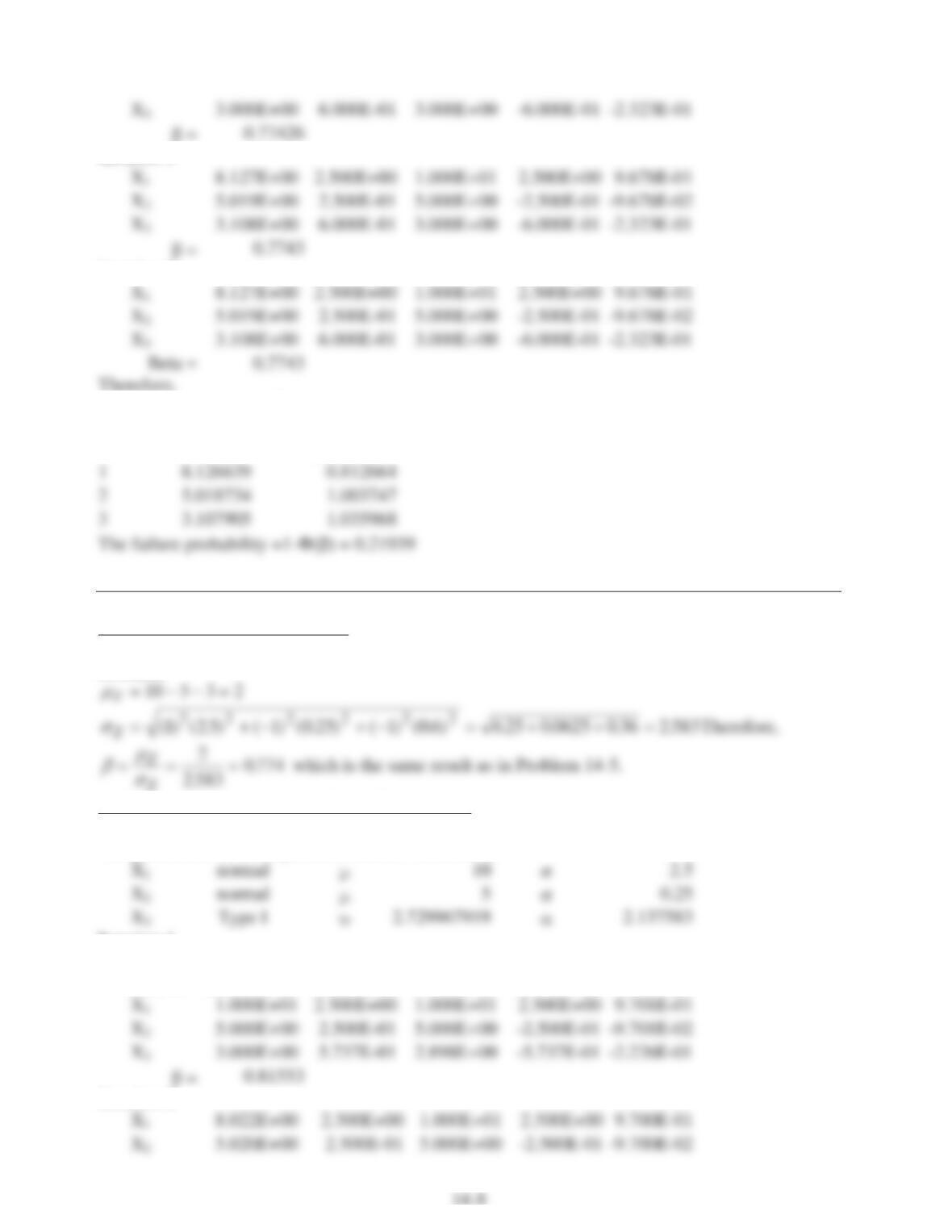
Using advanced second-moment reliability analysis, the following table can be constructed:
Iteration 1
Random Assumed Eq. Normal Eq. Normal Partial Direction
Variable Failure Point Std. Dev Mean Derivatives Cosines
Direct Simulation
0.6
0.7
t
Conditional Expectation Simulation
0.00002
0.000025
0.00003
t
Iteration 2
Iteration 3
E = 0.7743
Failure Point Partial Safety
Factors
Problem 14-6.
a. First-order Reliability Analysis
Using first-order reliability analysis based on first-order Taylor series, the following can be
obtained:
a. Advanced Second-moment Reliability Analysis
Using advanced second-moment reliability analysis, the following table can be constructed:
The parameters of the lognormal random variables are
Iteration 1
Random Assumed Eq. Normal Eq. Normal Partial Direction
Variable Failure Point Std. Dev Mean Derivatives Cosines
Iteration 2
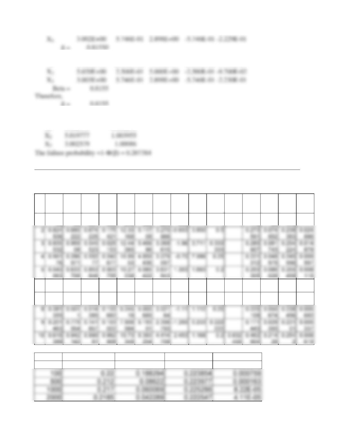
14-9
E = 0.81550
Iteration 3
X1 8.022E+00 2.500E+00 1.000E+01 2.500E+00 9.700E-01
E = 0.8155
Failure Point Partial Safety
Factors
X1 8.022355 0.802236
Problem 14-7.
The following table shows the results of 10 simulation cycles, in which X1 was used as the control
variable in the CE method:
i u1 u2 u3 u4 x1 x2 x3 W z PF
Direct
COV(
Pf
Direct)
Pfi for
CE
Pfi^2
for CE
Mean(
Pf CE)
COV(
Pf CE)
1 0.017
33
0.413
54
0.584
637
0.747
438
4.719
246
4.945
388
3.128
263
0.666
448
-3.288 1 0.203
175
0.041
28
0.203
175
na
6 0.084
553
0.609
814
0.195
888
0.986
716
6.562
303
5.069
709
2.486
158
2.218 -0.774 0.333
333
0.159
702
0.025
505
0.239
498
0.008
891
7 0.324
347
0.624
732
0.703
092
0.795
43
8.861
057
5.079
483
3.319
99
0.825 0.544 0.285
714
0.245
552
0.060
296
0.240
363
0.006
964
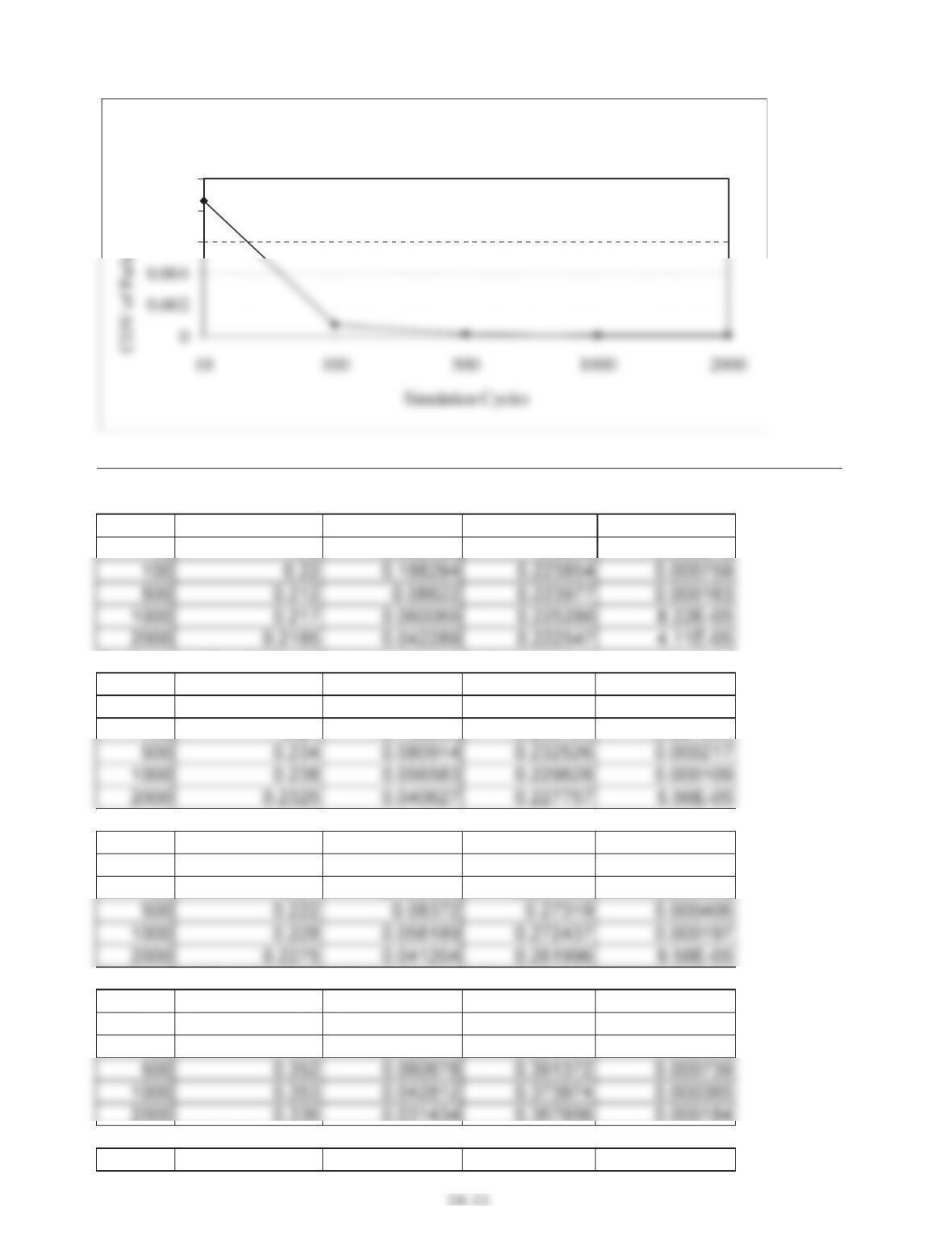
The results for different numbers of cycles are shown in the following table and figures:
N Direct, Mean Pf Direct, COV(Pf) CE, Mean Pf CE, COV(Pf)
10 0.2 0.632456 0.2542 0.008619
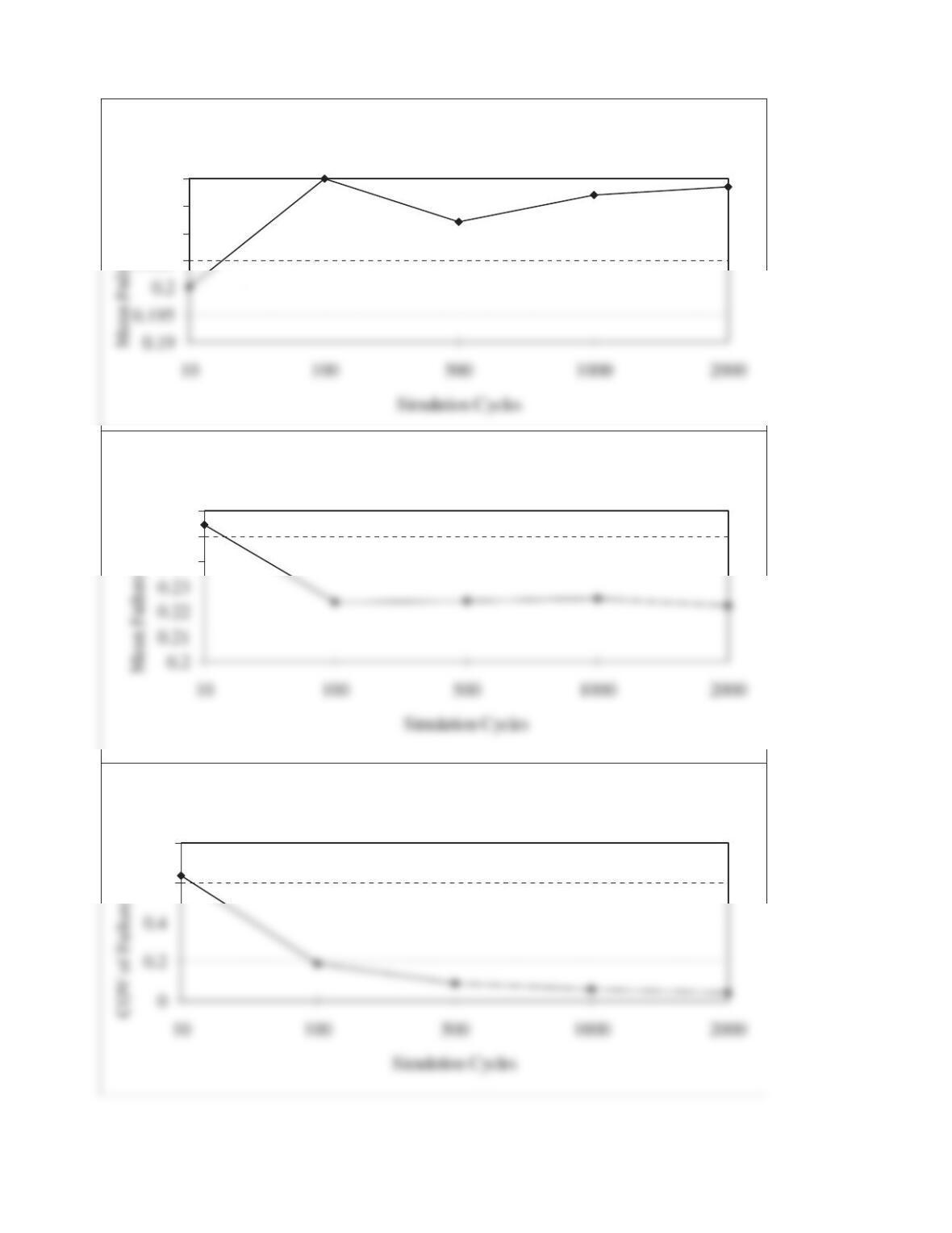
14-10
Direct Simulation
0.205
0.21
0.215
0.22
t
Conditional Expectation Simulation
0.24
0.25
0.26
t
Direct Simulation
0.6
0.8
t
Problem 14-8.
For I1 = 1, and I2 = 1, the following results are obtained:
N Direct, Mean Pf Direct, COV(Pf) CE, Mean Pf CE, COV(Pf)
10 0.2 0.632456 0.2542 0.008619
For I1 = 1, and I2 = 10, the following results are obtained:
N Direct, Mean Pf Direct, COV(Pf) CE, Mean Pf CE, COV(Pf)
10 0.3 0.483046 0.264896 0.010764
100 0.21 0.193956 0.235134 0.001084
For I1 = 5, and I2 = 1, the following results are obtained:
N Direct, Mean Pf Direct, COV(Pf) CE, Mean Pf CE, COV(Pf)
10 0.2 0.632456 0.258168 0.009224
100 0.21 0.193956 0.264454 0.001849
For I1 = 5, and I2 = 10, the following results are obtained:
N Direct, Mean Pf Direct, COV(Pf) CE, Mean Pf CE, COV(Pf)
10 0.5 0.316228 0.410896 0.038799
100 0.4 0.122474 0.395187 0.00373
2000 0.336 0.031434 0.367856 0.000184
For I1 = 10, and I2 = 1, the following results are obtained:
N Direct, Mean Pf Direct, COV(Pf) CE, Mean Pf CE, COV(Pf)
Conditional Expectation Simulation
0.006
0.008
0.01
t
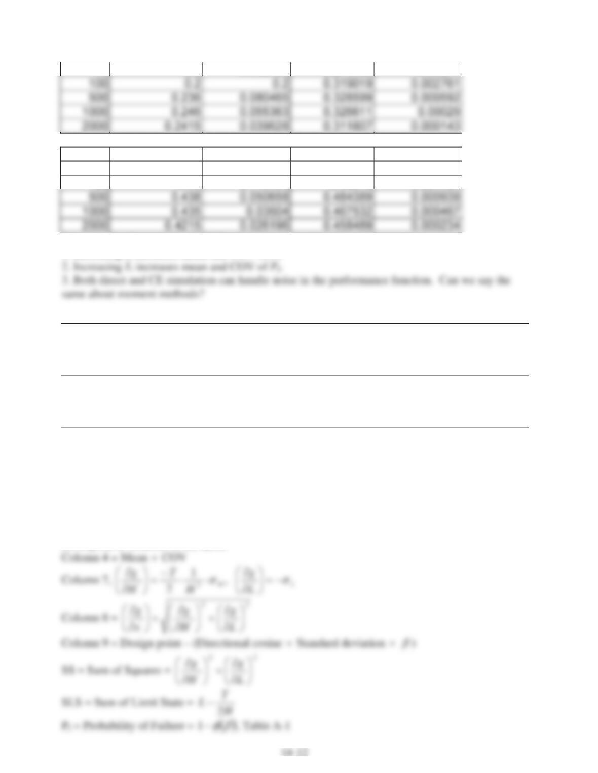
10 0.2 0.632456 0.270128 0.01271
For I1 = 10, and I2 = 10, the following results are obtained:
N Direct, Mean Pf Direct, COV(Pf) CE, Mean Pf CE, COV(Pf)
10 0.4 0.387298 0.492298 0.050872
100 0.43 0.115134 0.48015 0.004727
Based on the above results the following observations can be made:
1. Increasing I2 increases mean and COV of Pf.
Problem 14-9.
The results are similar to Problem 14-7.
Problem 14-10.
The results are similar to Problem 14-8.
Problem 14-11.
The performance function can be expressed as.
Z = L – T/(2H)
where T is a constant, and L and H are random variables. The advanced second moment method
can be used as provided below. Sample calculations are provided with a summary at the end for
all cases.
(a) Normal Distributions
The computations are summarized in the table below according to the following equations that
correspond to columns of the table:
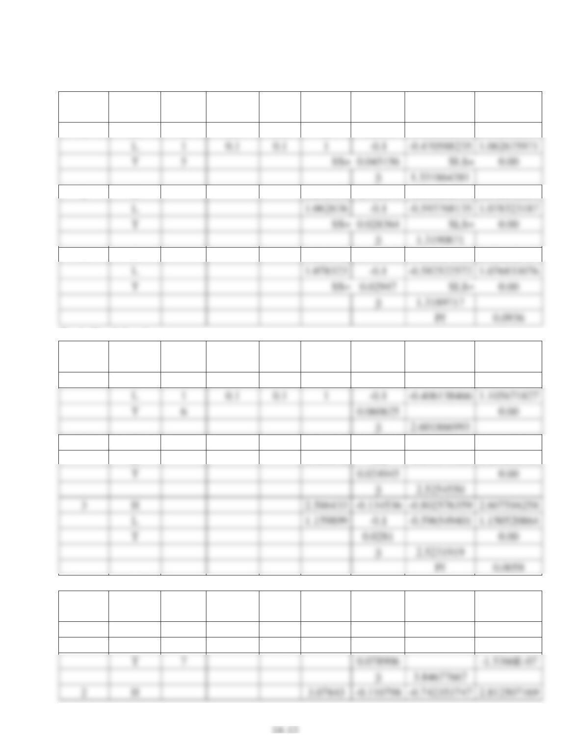
T = 5, H = 2, L = 1
(1) (2) (3) (4) (5) (6) (7) (8) (9)
Iteration
number
Random
Variable
Mean
Value
Standard
Deviation COV Design
Point
Partial
derivative
Directional
Cosine
New Design
Point
1 H 2 0.3 0.15 2 -0.1875 -0.882352941 2.352552336
2 H 2.352552 -0.135514 -0.804636192 2.318415559
3 H 2.318416 -0.139534 -0.812814526 2.321623797
T = 6, H = 2, L = 1
Iteration
number
Random
Variable
Mean
Value
Standard
Deviation COV Design
Point
Partial
derivative
Directional
Cosine
New Design
Point
1 H 2 0.3 0.15 2 -0.225 -0.913811549 2.713284832
2 H 2.713285 -0.122251 -0.774029868 2.586433282
L 1.105672 -0.1 -0.633149085 1.159898953
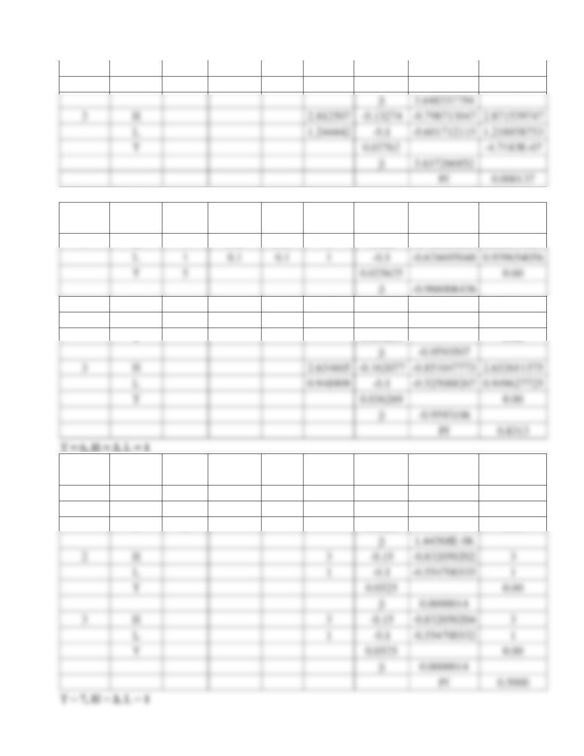
T = 7, H = 2, L = 1
Iteration
number
Random
Variable
Mean
Value
Standard
Deviation COV Design
Point
Partial
derivative
Directional
Cosine
New Design
Point
1 H 2 0.3 0.15 2 -0.2625 -0.934487735 3.078429685
L 1 0.1 0.1 1 -0.1 -0.355995328 1.136943452
14-14
L 1.136943 -0.1 -0.670008145 1.244441604
T 0.022276 -3.3164E-07
T = 5, H = 3, L = 1
Iteration
number
Random
Variable
Mean
Value
Standard
Deviation COV Design
Point
Partial
derivative
Directional
Cosine
New Design
Point
1 H 3 0.45 0.15 3 -0.125 -0.780868809 2.660554067
2 H 2.660554 -0.158931 -0.846395132 2.634604616
L 0.939654 -0.1 -0.532555424 0.948909259
T 0.035259 0.00
Iteration
number
Random
Variable
Mean
Value
Standard
Deviation COV Design
Point
Partial
derivative
Directional
Cosine
New Design
Point
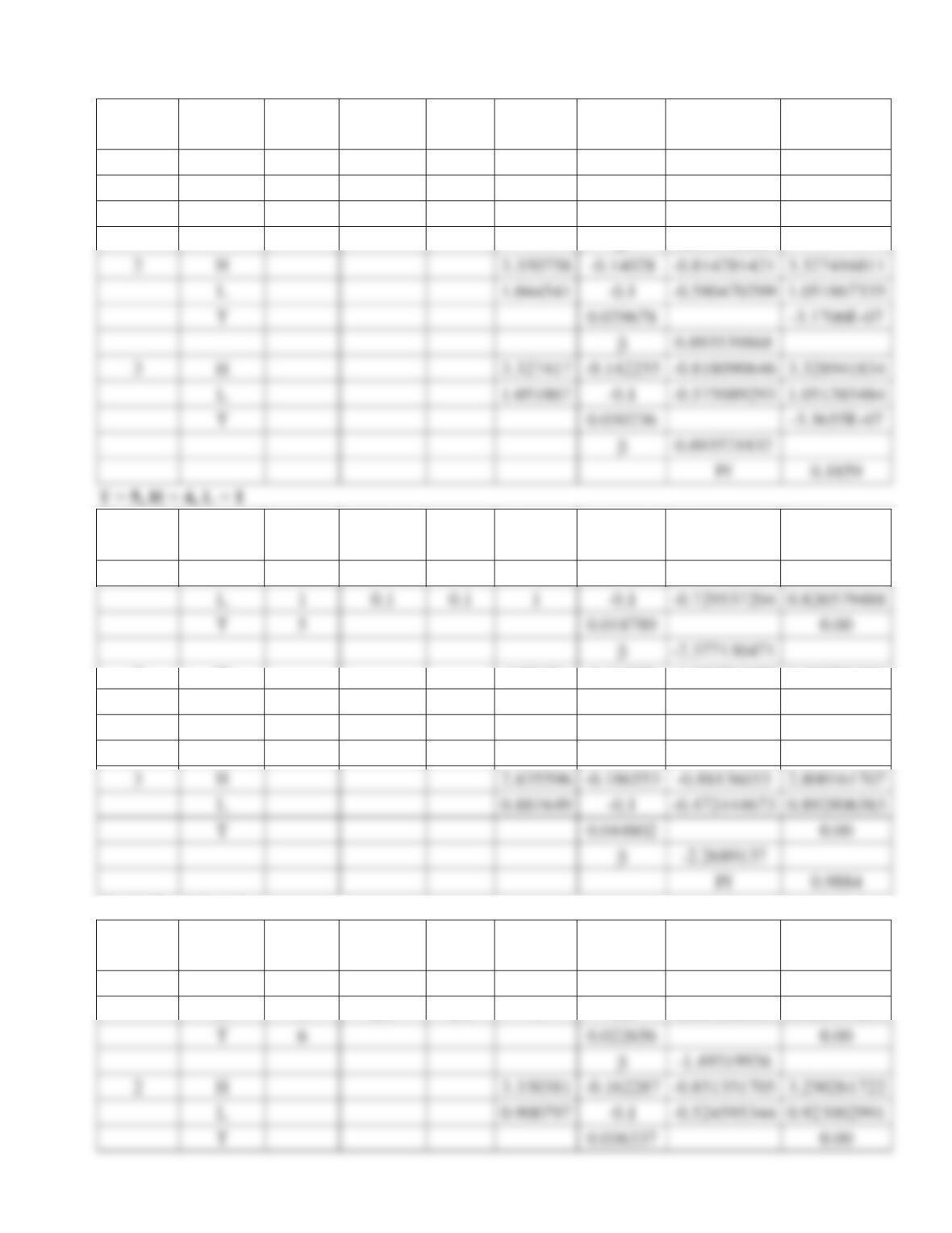
1 H 3 0.45 0.15 3 -0.15 -0.832050294 3
L 1 0.1 0.1 1 -0.1 -0.554700196 1
T 6 0.0325 0.00
14-15
Iteration
number
Random
Variable
Mean
Value
Standard
Deviation COV Design
Point
Partial
derivative
Directional
Cosine
New Design
Point
1 H 3 0.45 0.15 3 -0.175 -0.868243142 3.35075765
L 1 0.1 0.1 1 -0.1 -0.496138938 1.044540654
T 7 0.040625 -7.7202E-07
E 0.897745581
Iteration
number
Random
Variable
Mean
Value
Standard
Deviation COV Design
Point
Partial
derivative
Directional
Cosine
New Design
Point
1 H 4 0.6 0.15 4 -0.09375 -0.683941129 3.024509621
2 H 3.02451 -0.163976 -0.853762855 2.835596023
L 0.826579 -0.1 -0.520662066 0.881649224
T 0.036888 0.00
E -2.2730824
T = 6, H = 4, L = 1
Iteration
number
Random
Variable
Mean
Value
Standard
Deviation COV Design
Point
Partial
derivative
Directional
Cosine
New Design
Point
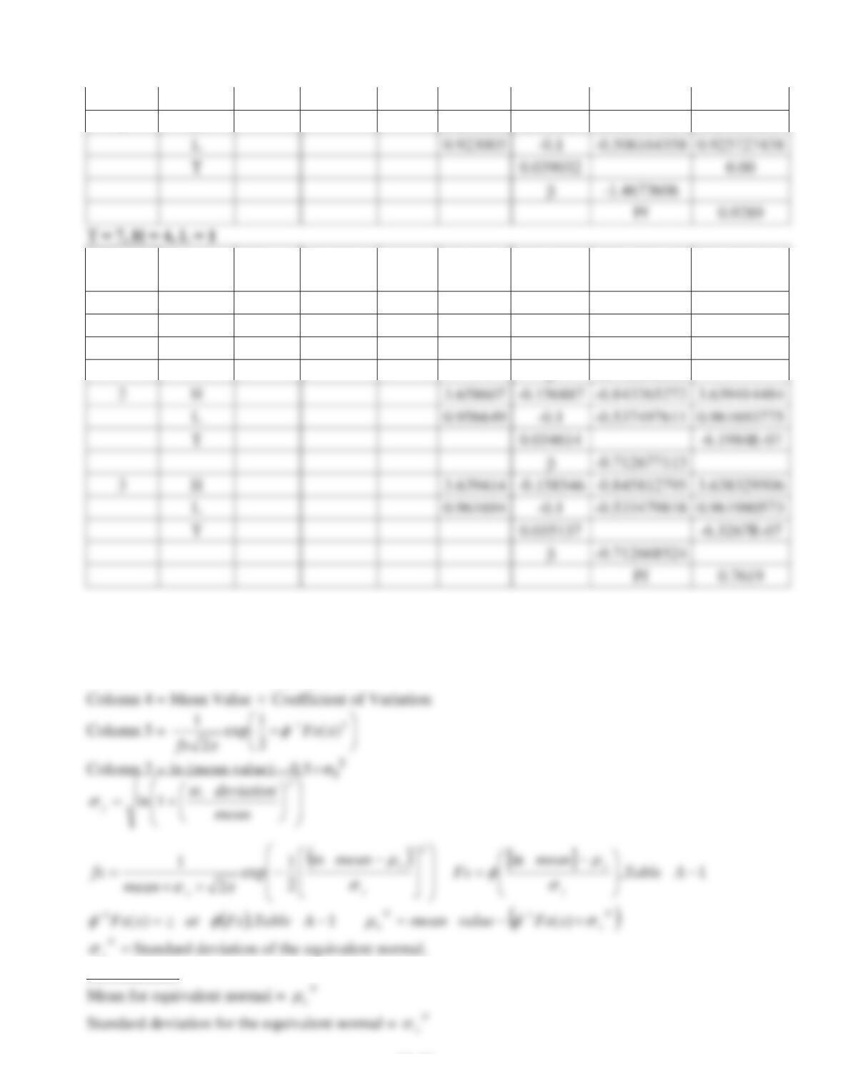
1 H 4 0.6 0.15 4 -0.1125 -0.747409319 3.33038133
L 1 0.1 0.1 1 -0.1 -0.664363839 0.900797234
14-16
E -1.4677410
3 H 3.250262 -0.170387 -0.862437037 3.24069634
Iteration
number
Random
Variable
Mean
Value
Standard
Deviation COV Design
Point
Partial
derivative
Directional
Cosine
New Design
Point
1 H 4 0.6 0.15 4 -0.13125 -0.79543172 3.658607403
L 1 0.1 0.1 1 -0.1 -0.606043215 0.956648559
T 7 0.027227 -4.1011E-07
E -0.715319301
(b) Lognormal Distributions
The computations are summarized in the table below according to the following equations that
correspond to columns of the table:
Column 3 = Mean Value – [ )(
1xFxfx
u
I
]
x
For iterations:
14-17
New design point = Mean for equivalent normal – (Directional cosine u Standard deviation of
equivalent normal u
E
)
T=5 H=2 L=1
(1) (2) (3) (4) (5) (6) (7)
Random
variable
Mean
Value
Mean for
equivalent
Normal
Standard
Deviation
Standard
Deviation of
Equivalent
Normal
Coefficient of
Variation Py
H 2 1.90054154 0.3 0.2983328 0.15 0.682022
Vy
Lognormal
Distribution,
fx
Lognormal
Cumulative,
Fx
)-1(Fx(x*)) Px
N Vx
N
Iteration Random
variable
Mean for
equivalent
normal
Standard
deviation for
equivalent
normal
Partial
derivative
Directional
cosine
New
design
point
H 1.97774941 0.298332762 -0.190677 -0.8860742 2.355892
Lognormal
Distribution,
fx
Lognormal
Cumulative,
Fx
)-1(Fx(x*)) Px
N Vx
N
0.57089856 0.879501844 1.1725001 1.94385218 0.35142
14-18
Iteration Random
variable
Mean for
equivalent
normal
Standard
deviation for
equivalent
normal
Partial
derivative
Directional
cosine
New
design
point
H 1.94385218 0.351420051 -0.232509 -0.9101199 2.376071
Lognormal
Distribution,
fx
Lognormal
Cumulative,
Fx
)-1(Fx(x*)) Px
N Vx
N
0.52848287 0.89059065 1.2296755 1.94023686 0.35443
0.088287
Iteration Random
variable
Mean for
equivalent
normal
Standard
deviation for
equivalent
normal
Partial
derivative
Directional
cosine
New
design
point
H 1.94023686 0.354429951 -0.235375 -0.9133171 2.378128
Lognormal
Distribution,
fx
Lognormal
Cumulative,
Fx
)-1(Fx(x*)) Px
N Vx
N
0.52426277 0.891673614 1.2354781 1.93985862 0.354737
T=5 H=3 L=1
Random
variable
Mean
Value
Mean for
equivalent
Normal
Standard
Deviation
Standard
Deviation of
Equivalent
Normal
Coefficient of
Variation Py
H 3 2.93369436 0.45 0.4474991 0.15 1.087487
Iteration Random
variable
Mean for
equivalent
normal
Standard
deviation for
equivalent
normal
Partial
derivative
Directional
cosine
New
design
point
H 2.96662412 0.447499143 -0.127118 -0.7867003 2.657086
Lognormal
Distribution,
fx
Lognormal
Cumulative, Fx )-1(Fx(x*)) Px
N Vx
N
0.76594143 0.229906869 -0.739153 2.9500482 0.396348
Iteration Random
variable
Mean for
equivalent
normal
Standard
deviation for
equivalent
normal
Partial
derivative
Directional
cosine
New
design
point
H 2.9500482 0.396348002 -0.113857 -0.7716315 2.665347
Lognormal
Distribution,
fx
Lognormal
Cumulative, Fx )-1(Fx(x*)) Px
N Vx
N
0.77523498 0.236272389 -0.718344 2.95094607 0.39758
Iteration Random
variable
Mean for
equivalent
normal
Standard
deviation for
equivalent
normal
Partial
derivative
Directional
cosine
New
design
point
H 2.95094607 0.397580269 -0.114141 -0.7733762 2.664777
Lognormal
Distribution,
fx
Lognormal
Cumulative, Fx )-1(Fx(x*)) Px
N Vx
N
0.77460258 0.235831253 -0.719776 2.9508851 0.397495
14-20
Pf
0.823994
T=5 H=4 L=1
Random
variable
Mean
Value
Mean for
equivalent
Normal
Standard
Deviation
Standard
Deviation of
Equivalent
Normal
Coefficient of
Variation Py
H 4 3.95027077 0.6 0.5966655 0.15 1.375169
Vy
Lognormal
Distribution,
fx
Lognormal
Cumulative, Fx )-1(Fx(x*)) Px
N Vx
N
0.149166 0.66676257 0.529726894 0.0745831 3.95549883 0.596666
Iteration Random
variable
Mean for
equivalent
normal
Standard
deviation for
equivalent
normal
Partial
derivative
Directional
cosine
New
design
point
H 3.95549883 0.596665524 -0.095339 -0.6909357 3.012053
Lognormal
Distribution,
fx
Lognormal
Cumulative, Fx )-1(Fx(x*)) Px
N Vx
N
0.16728111 0.033839638 -1.827138 3.83297634 0.449295
Iteration Random
variable
Mean for
equivalent
normal
Standard
deviation for
equivalent
normal
Partial
derivative
Directional
cosine
New
design
point
H 3.83297634 0.449294614 -0.076454 -0.6784178 3.040187
Lognormal
Distribution,
fx
Lognormal
Cumulative, Fx )-1(Fx(x*)) Px
N Vx
N
0.18536303 0.038797933 -1.764811 3.84051404 0.453492