Chapter 14: Computational Engineering Tools Electronic Spreadsheets
14.1 Using the Excel Help menu, discuss how the following functions are used. Create
a simple example and demonstrate the proper use of the function.
(a) TRUNC(number,num_digits)
(b) ROUND(number,num_digits)
(c) COMBIN(number,number_chosen)
(d) DEGREES(angle)
(e) SLOPE(known_y’s,known_x’s)
(f) CEILING(number,significance)
176
© 2020 Cengage Learning®. All Rights Reserved. May not be scanned, copied or duplicated, or posted to a publicly accessible website,
in whole or in part.
Rounds up to the nearest given significance.
Examples: CEILING(3.04,0.1) = 3.1; CEILING(3.4,1) = 4
14.2 In Chapter 20, we will cover engineering economics. For now, using the Excel
Help menu, familiarize yourself with the following functions. Create a simple
example and demonstrate the proper use of the function.
(a) FV(rate, nper, pmt, pv, type)
(b) IPMT(rate, per, nper, pv, fv, type)
(c) NPER(rate, pmt, pv, fv, type)
(d) PV(rate, nper, pmt, fv, type)
177
© 2020 Cengage Learning®. All Rights Reserved. May not be scanned, copied or duplicated, or posted to a publicly accessible website,
in whole or in part.
assumed to be 0 (zero); type is the number 0 or 1 indicating when payments are
due, end or the beginning of period.
Example: If you were to put $6710.08 in an account that pays 8% annually, over
how many periods (years) you can withdraw $1000?
NPER(8%,1000,-6710.08,0,0) = 10 See also next example.
(d) PV(rate,nper,pmt,fv,type)
Returns the present value of a series of payments.
rate: interest rate per period; nper: total number of payment periods in an
annuity; Pmt: payment made each period; Pv: present value, or the lump-sum
amount that a series of future payments is worth right now. If pv is omitted, it is
assumed to be 0 (zero); type is the number 0 or 1 indicating when payments are
due, end or the beginning of period.
Example: The present value of $1000 deposits every year for 10 years at 8%
interest rate is: PV(8%,10,-1000,0,0) = $6710.08. In other word, today, if you
were to put $6710.08 in an account that pays 8% annually, you can withdraw
$1000 every year for the next 10 years.
14.3 In Chapter 10, we discussed fluid pressure and the role of water towers in small
towns. Recall that the function of a water tower is to create a desirable municipal
water pressure for household use and other usage in a town. To achieve this
purpose, water is stored in large quantities in elevated tanks. Also recall that the
municipal water pressure may vary from town to town, but it generally falls
somewhere between 50 and 80 lb/in2 (psi). In this assignment, use Excel to create
a table that shows the relationship between the height of water above ground in
the water tower and the water pressure in a pipe line located at the base of the
water tower. The relationship is given by:
ghP
where
P = the water pressure at the base of the water tower (lb/ft2)
= the density of water, (rho) = 1.94 slugs/ft3
g = the acceleration due to gravity, g = 32.3 ft/s2
h = is the height of water above ground in feet (ft)
Create a table that shows the water pressure in a pipe located at the base of the
water tower as you vary the height of water in increments of 10 ft. Also plot water
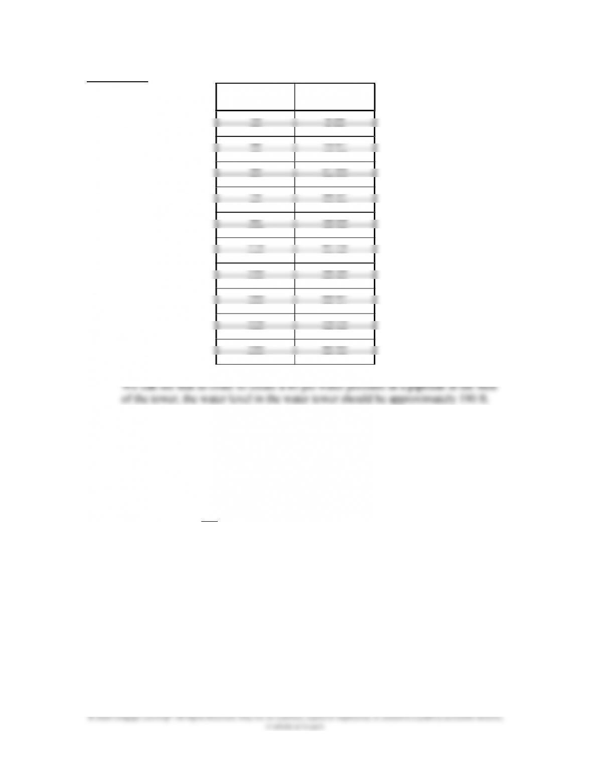
pressure vs. the height of water in feet. What should be the water level in the
water tower to create 80 psi water pressure in a pipe at the base of the water
tower?
178
SOLUTION
Water level Water Pressure
in the tower (ft) (lb/in2)
20 8.68
40 17.35
60 26.03
80 34.70
100 43.38
120 52.06
140 60.73
160 69.41
180 78.08
200 86.76
14.4 As we explained in Chapter 10, viscosity is a measure of how easily a fluid flows.
For example, honey has a higher value of viscosity than does water because if you
were to pour water and honey side by side on an inclined surface, the water will
flow faster. The viscosity of a fluid plays a significant role in the analysis of many
fluid dynamics problems. The viscosity of water can be determined from the
following correlation
)(
1
3
2
10 cT
c
c
where
viscosity (N·s/m2)
T temperature (K)
c1 2.414 x 10⁻⁵(N/s·m2)
c2 247.8 K
c3 140 K
Using Excel, create a table that shows the viscosity of water as a function of
temperature in the range of 0 C (273.15 K) to 100 C (373.15 K) in increments
of 5 C. Also create a graph showing the value of viscosity as a function of
temperature.
179
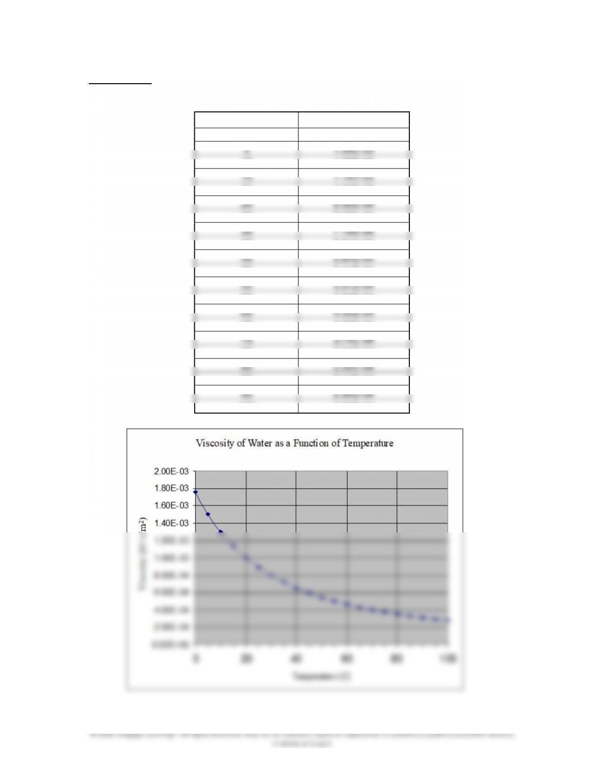
SOLUTION
Viscosity of water as a function of temperature
Temperature (C) Viscosity (N·s/m2)
0 1.75E-03
10 1.30E-03
20 1.00E-03
30 7.97E-04
40 6.51E-04
50 5.44E-04
60 4.63E-04
70 4.00E-04
80 3.51E-04
90 3.11E-04
100 2.79E-04

180
14.5 Using Excel, create a table that shows the relationship between the units of
temperature in degrees Celsius and Fahrenheit in the range of –50C to 150C.
Use increments of 10C.
SOLUTION
Temperature (°C)
Temperature (°F)
Temperature (°C)
Temperature (°F)
-45 -49 60 140
-35 -31 70 158
-25 -13 80 176
-15 5 90 194
-5 23 100 212
0 32 105 221
5 41 110 230
14.6 Using Excel, create a table that shows the relationship among the units of height
of people in centimeters, inches, and feet in the range of 150 cm to 2 m. Use
increments of 5 cm.
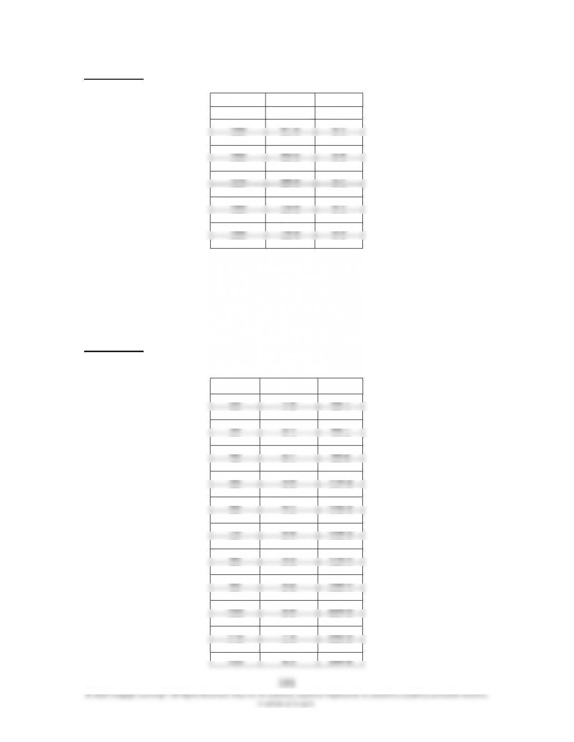
SOLUTION
Height (cm)
Height (in)
Height (ft)
150 59.1 4.9
160 63.0 5.2
170 66.9 5.6
180 70.9 5.9
190 74.8 6.2
200 78.7 6.6
14.7 Using Excel, create a table that shows the relationship among the units of mass to
describe people’s mass in kilogram, slugs, and pound mass in the range of 20 kg
to 120 kg. Use increments of 5 kg.
SOLUTION
mass (kg)
mass (slugs)
mass (lbm)
25 1.7 55.1
35 2.4 77.2
45 3.1 99.2
55 3.8 121.3
65 4.5 143.3
75 5.1 165.3
85 5.8 187.4
95 6.5 209.4
105 7.2 231.5
115 7.9 253.5

182
14.8 Using Excel, create a table that shows the relationship among the units of pressure
in Pa, psi, and inches of water in the range of 1000 Pa to 10,000 Pa. Use
increments of 500 Pa.
SOLUTION
Pressure (Pa)
Pressure (psi)
Pressure (inches of water)
1000 0.15 4.01
2000 0.29 8.03
3000 0.44 12.04
4000 0.58 16.06
5000 0.73 20.07
6000 0.87 24.09
7000 1.02 28.10
8000 1.16 32.12
9000 1.31 36.13
10000 1.45 40.15
14.9 Using Excel, create a table that shows the relationship between the units of
pressure in Pa and psi in the range of 10 kPa to 100 kPa. Use increments of
5 kPa.

183
SOLUTION
Pressure (kPa)
Pressure (psi)
15 2.18
25 3.63
35 5.08
45 6.53
55 7.98
65 9.43
75 10.88
85 12.33
95 13.78
14.10 Using Excel, create a table that shows the relationship between the units of power
in watts and horsepower in the range of 100 Watts to 10,000 Watts. Use smaller
increments of 100 W up to 1000 W, and then use increments of 1000 W all the
way up to 10,000 W.

184
SOLUTION
Power (W) Power (hp)
100 0.13
300 0.40
500 0.67
700 0.94
900 1.21
2000 2.68
4000 5.36
6000 8.05
8000 10.73
10000 13.41
185
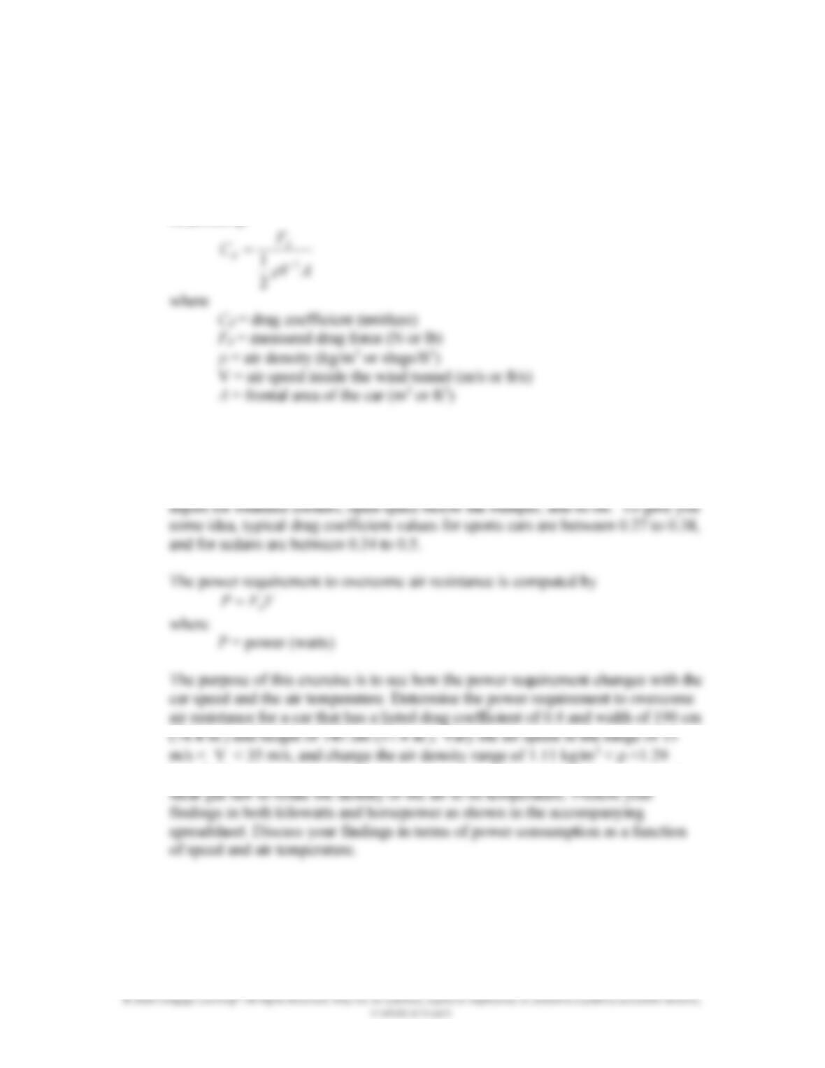
14.11 As we explained in Chapter 7, the air resistance to motion of a vehicle is
something important that engineers investigate. As you may also know, the drag
force acting on a car is determined experimentally by placing the car in a wind
tunnel. The air speed inside the tunnel is changed, and the drag force acting on the
car is measured. For a given car, the experimental data is generally represented by
a single coefficient that is called drag coefficient. It is defined by the following
relationship:
F
Cd
d
2
1
The frontal area A represents the frontal projection of the car’s area and could be
approximated simply by multiplying 0.85 times the width and the height of a
rectangle that outlines the front of a car. This is the area that you see when you
view the car from a direction normal to the front grills. The 0.85 factor is used to
kg/m3. The given air density range corresponds to 0C to 45C. You may use the
186
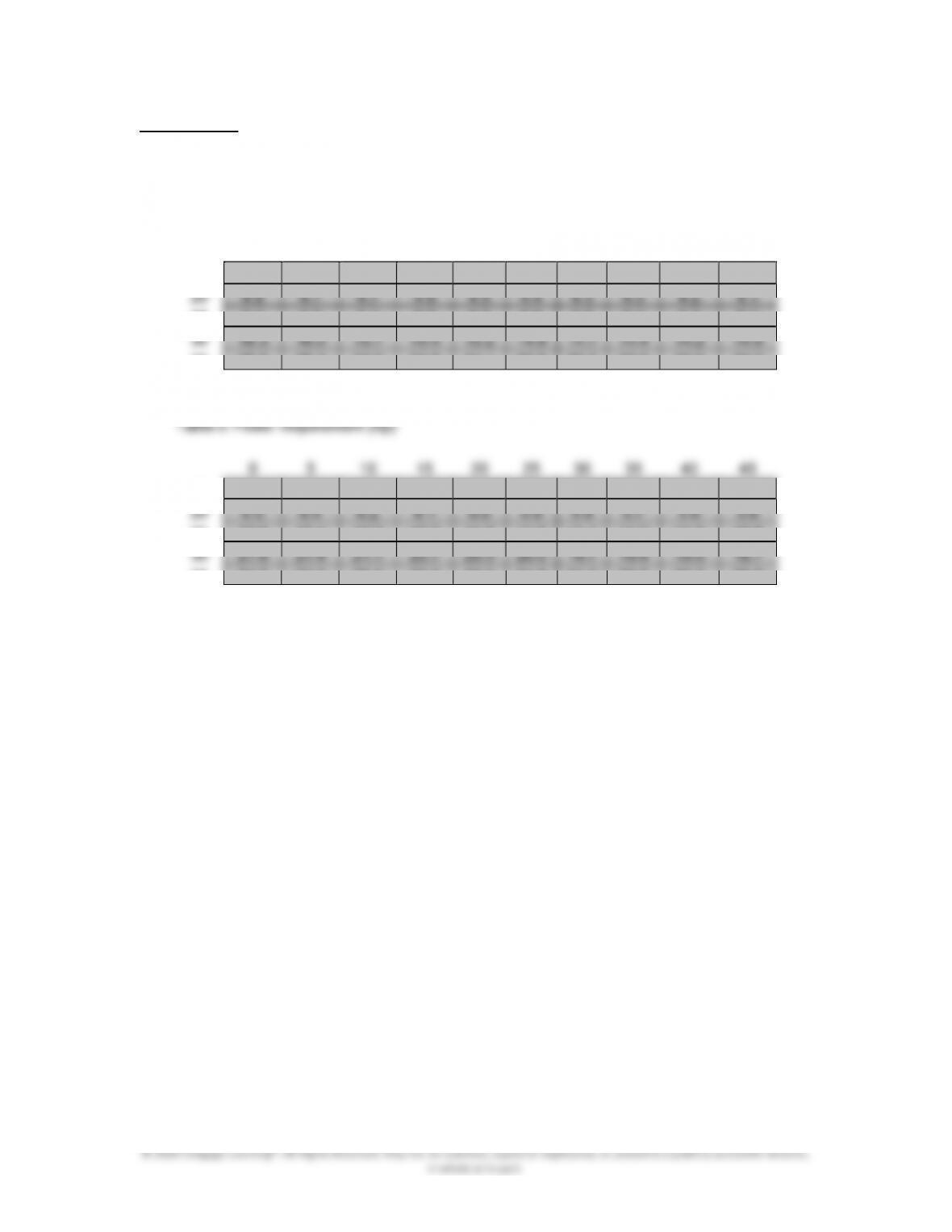
SOLUTION
Table-1 Power requirement (kW)
Car
Ambient Temperature (C)
speed
(m/s)
0 5 10 15 20 25 30 35 40 45
15 2.0 2.0 2.0 1.9 1.9 1.9 1.8 1.8 1.8 1.7
25 9.4 9.3 9.1 8.9 8.8 8.6 8.5 8.4 8.2 8.1
35 25.9 25.4 24.9 24.5 24.1 23.7 23.3 22.9 22.6 22.2
15 2.7 2.7 2.6 2.6 2.5 2.5 2.5 2.4 2.4 2.3
25 12.6 12.4 12.2 12.0 11.8 11.6 11.4 11.2 11.0 10.8
35 34.7 34.0 33.4 32.9 32.3 31.8 31.2 30.7 30.2 29.8
187
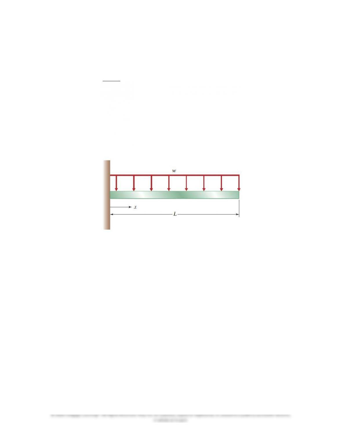
14.12 The cantilevered beam shown in the accompanying figure is used to support a
load acting on a balcony. The deflection of the centerline of the beam is given by
the following equation
)64(
24
22
2
LLxx
EI
wx
y
where
y = deflection at a given x location (m)
w = distributed load (N/m)
E = modulus of elasticity (N/m2)
I = second moment of area (m4)
x = distance from the support as shown (x)
L = length of the beam (m)
Using Excel, plot the deflection of a beam whose length is 5 m with the modulus
of elasticity of E = 200 GPa and I = 99.1 x 106 mm4. The beam is designed to
carry a load of 10,000 N/m. What is the maximum deflection of the beam?
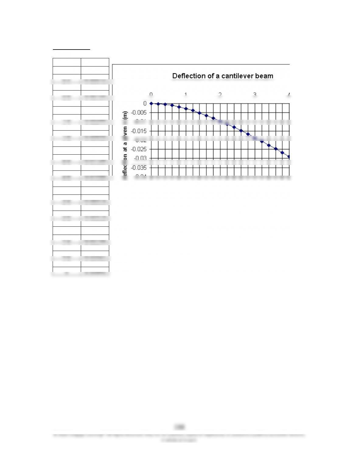
SOLUTION
x (m) y (m)
0 0
0.4 -0.00048
0.8 -0.00181
1 -0.00275
1.4 -0.00511
1.8 -0.00799
2 -0.00959
2.4 -0.01305
2.8 -0.01678
3 -0.01873
3.4 -0.02274
3.8 -0.02685
4 -0.02893
4.4 -0.03311
4.8 -0.03732
189
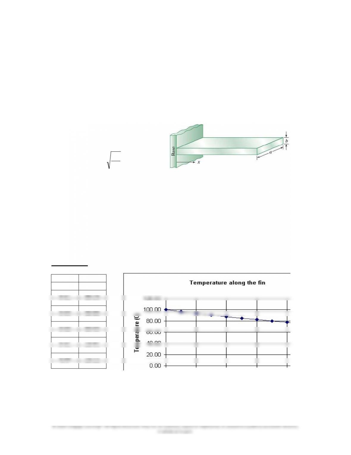
14.13 Fins, or extended surfaces, are commonly used in a variety of engineering
applications to enhance cooling. Common examples include a motorcycle or lawn
mower engine head, extended surfaces used in electronic equipment, and finned
tube heat exchangers in room heating and cooling applications. Consider a
rectangular profile of aluminum fins shown in the accompanying figure, which are
used to remove heat from a surface whose temperature is 100C ( base
T=100C).
The temperature of the ambient air is 20C. We are interested in determining how
the temperature of the fin varies along its length and plotting this temperature
variation. For long fins, the temperature distribution along the fin is given by:
mx
ambientbaseambient eTTTT
)(
where
kA
hp
m
h = the heat transfer coefficient, W/m2.K
p = perimeter of the fin 2*(a+b), m
A = cross-sectional area of the fin (a*b), m2
k = thermal conductivity of the fin material, W/m.K
Plot the temperature distribution along the fin using the following data:
k = 168 W/m·K, h = 12 W/m2·K, a = 0.05 m, b = 0.01 m. Vary x from 0 to 0.01
m in increments of 0.01 m.
SOLUTION
x (m) T (°C)
0 100.00
0.02 93.64
0.04 87.79
0.06 82.40
0.08 77.44
0.1 72.88