13-17
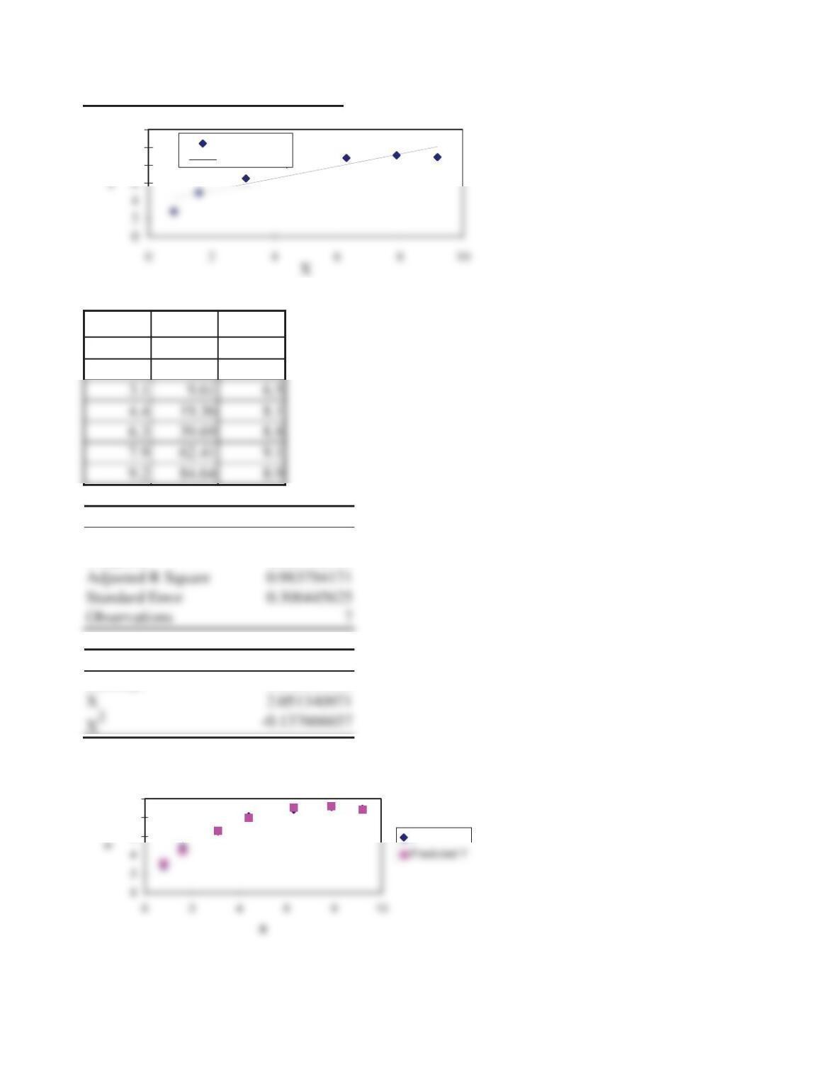
Slope 0.686053651
8
10
12
Y
Predicted Y
For the quadratic model, the following table will be used:
X1 = X X2 = X2Y
0.8 0.64 2.8
1.6 2.56 4.9
Regression Statistics
Multiple R 0.994583387
R Square 0.989196114
Coefficients
Intercept 1.560993356
X Line Fit Plot
6
8
10
Y
13-18
X^2 Line Fit Plot
6
8
10
X^2
Y
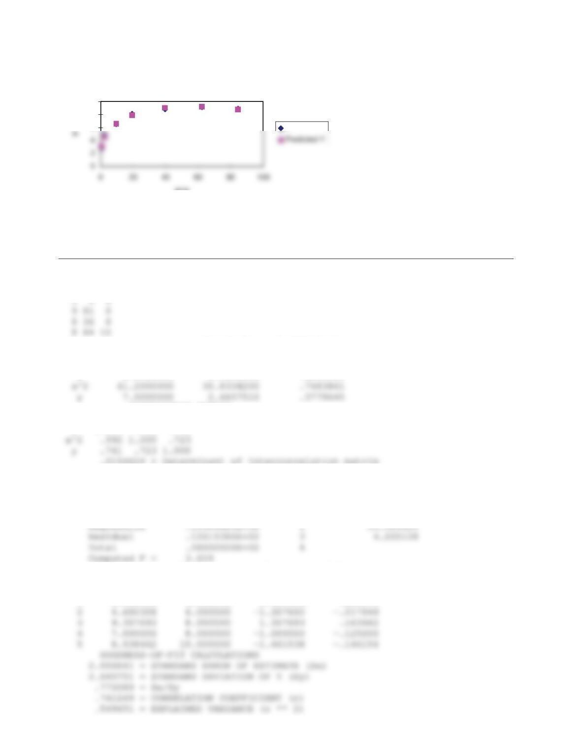
The quadratic model is better than the linear model as shown in the figures. Also, the regression
statistics for the quadratic model are better than the statistics of the linear model.
Problem 13-38.
x x^2 Y
4 16 3
Standard Coefficient
Var Mean Deviation of Variation
— ———— ———– ————
x 6.0000000 2.5495100 .4249183
CORRELATION MATRIX
1 2 3
x 1.000 .992 .741
.0154624 = Determinant of intercorrelation matrix
LINEAR MODEL
Y = 2.384615 + 0.7692308 * X
ANALYSIS OF VARIANCE TABLE
Source Sum of squares df Mean square
———- ————– — ———–
Predicted Observed Error Relative
I YP Y e = YP – Y Error(e/Y)
— ———- ———- ———- ———-
1 5.461538 3.000000 2.461538 .820513
13-19
QUADRATIC MODEL
Var b t R R**2 t*R
OBS PREDICTED OBSERVED RESIDUAL REL ERROR
NO. YP Y e = YP – Y e / Y
— ———— ———– ———– ———-
1 5.5431790 3.0000000 2.5431790 .84773
GOODNESS-OF-FIT STATISTICS
.5591688 = MULTIPLE R SQUARE
.7477759 = MULTIPLE R
Problem 13-39.
x x^2 x^3 Y
2 4 8 1.7
Standard Coefficient
Var Mean Deviation of Variation
— ———— ———– ————
X 6.0000000 3.1622780 .5270463
CORRELATION MATRIX
1 2 3 4
X 1.000 .981 .943 .989
ANALYSIS OF VARIANCE TABLE
Source Sum of squares df Mean square
Predicted Observed Error Relative
13-20
I YP Y e = YP – Y Error(e/Y)
— ———- ———- ———- ———-
1 1.220000 1.700000 -.480000 -.282353
QUADRATIC MODEL
Var b t R R**2 t*R
— ———– ——– ——- ——- ——-
OBS PREDICTED OBSERVED RESIDUAL REL ERROR
NO. YP Y e = YP – Y e / Y
— ———— ———– ———– ———-
1 1.6914290 1.7000000 -.0085715 -.00504
CUBIC MODEL
Var b t R R**2 t*R
— ———– ——– ——- ——- ——-
X .1095348 .11834 .98857 .97727 .11699
OBS PREDICTED OBSERVED RESIDUAL REL ERROR
NO. YP Y e = YP – Y e / Y
— ———— ———– ———– ———-
1 1.7020000 1.7000000 .0019996 .00118
2 2.7946760 2.8000000 -.0053236 -.00190
13-21
Problem 13-40.
Standard Coeff. of
Var Mean deviation variation
— ——— ——— ———
X .000000 1.581139 .000000
CORRELATION MATRIX
Var 1 2 3 4
X 1.000 .000 .943 .955
According to the partial F statistic the linear model is more important than
the quadratic or cubic.
y = 0.398 – 1.8 * x
-1.800000 = Intercept
Obs. Predicted Measured Error Relative
No. YP Y e = YP – Y error (e/Y)
—- ———— ———— ———— ———–
1 -2.596000 -2.360000 -.236000 .1000
5 -1.004000 -.840000 -.164000 .1952
GOODNESS-OF-FIT STATISTICS
————————–
.9119 = Increase in R**2 Due to Variable Added
.9119 = Multiple R**2
The partial F test suggests that the quadratic term is the next most
important. When it is added the following are the results:
y = -2 + 0.398 x + 0.1 x ^ 2
Var b t r r**2 t*r Se(bi) Se(bi)/bi
— ——— —— —– —– —– ——– ———
Partial R Partial F
Var to enter to enter
— ——— ———
2 .9567 21.608
13-22
GOODNESS-OF-FIT STATISTICS
.0806 = Increase in R**2 Due to Variable Added
.9925 = Multiple R**2
Adding the quadratic term increased the explaned variance by 8.1% and caused
the standard error ratio to decrease from 0.343 to 0.122, which is generally
considered a significant improvement.
CUBIC MODEL
ERROR ANALYSIS
============================================================
Obs. Predicted Measured Error Relative
No. YP Y e = YP – Y error (e/Y)
—- ———— ———— ———— ———–
1 -2.360000 -2.360000 .000000 .0000
2 -2.370000 -2.370000 .000000 .0000
Problem 13-41.
DATA MATRIX
1 1 5
Standard Coefficient
Var Mean Deviation of Variation
— ———— ———– ————
X 3.5000000 1.8708290 .5345225
13-23
2.7000090 = Intercept
OBS PREDICTED OBSERVED RESIDUAL REL ERROR
NO. YP Y e = YP – Y e / Y
— ———— ———– ———– ———-
1 5.2500090 5.0000000 .2500086 .05000
2 7.8357210 8.0000000 -.1642790 -.02053
Problem 13-42.
Model
R
2
R
Partial F 2
X
05.0
F Total F 1
X
2
X
05.0
F
Linear 0.53 0.2809 8.594 22 4.30 8.594 1 22 4.30
cubic model is selected.
Problem 13-43.
Model
R
2
R
Partial F 2
X
05.0
F Total F 1
X
2
X
05.0
F
Linear 0.41 0.1681 1.819 9 5.12 1.819 1 9 5.12
Problem 13-44.
Model
R
2
R
Partial F 2
X
05.0
F Total F 1
X
2
X
05.0
F
Linear 0.47 0.2209 4.537 16 4.49 4.537 1 16 4.49
Quadratic 0.58 0.3364 7.604 15 4.54 3.802 2 15 3.68
13-24
The partial and total F stats for the linear and quadratic models are significant at 5%. For the cubic
Problem 13-45.
Y
aX b
Let
ZYca W X
ln , ln ln , and
Then
Z
i=1
i=1
i=1
The resulting derivatives are
Rearranging above two equations, the following set of normal equations can be obtained:
The coefficient a can be determined using
ae
c
X Y W(lnX) Z(lnY) W Z W2
1 1 0 0 0 0
2 1 0.69315 0 0 0.48045
13-25
Problem 13-46.
Making the logarithmic transform
21
lnlnlnln
xcxbay
Problem 13-47.
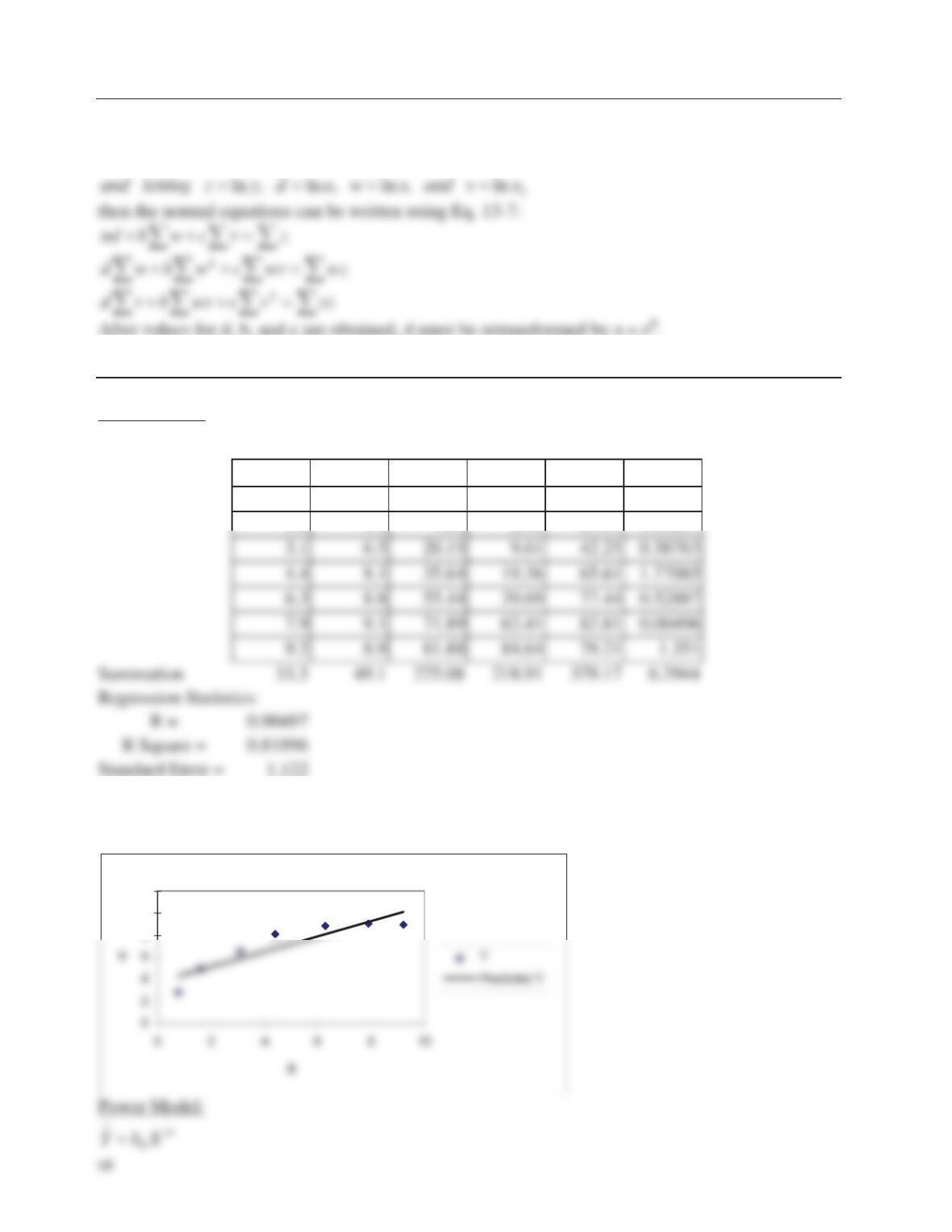
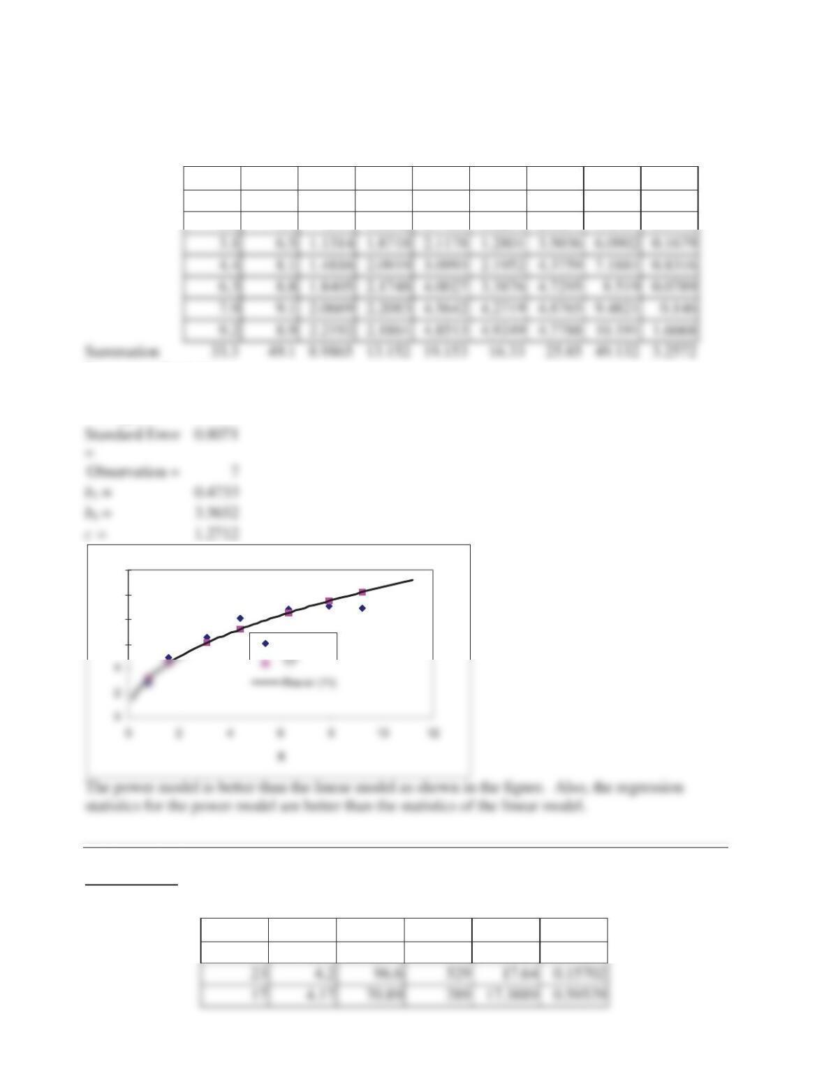
Linear Model:
Yb bX
01
X Y
XiYi Xi2Yi2(Yi^–Yi)2
0.8 2.8 2.24 0.64 7.84 2.24842
1.6 4.9 7.84 2.56 24.01 0.00267
Observation = 7
b1 = 0.68605
b0 = 3.75063
8
10
12
13-26
ZcbW
1
where
ZYcb W X
ln , ln , ln and
0
Xi Yi Wi(lnXi)Zi(lnYi)Wi Zi Wi2Zi2Yi
^
(Yi^–Yi)2
0.8 2.8 -0.223 1.0296 -0.23 0.0498 1.0601 3.2079 0.1664
1.6 4.9 0.47 1.5892 0.7469 0.2209 2.5257 4.4534 0.1995
Regression Statistics:
R = 0.9701
R Square = 0.9411
Problem 13-48.
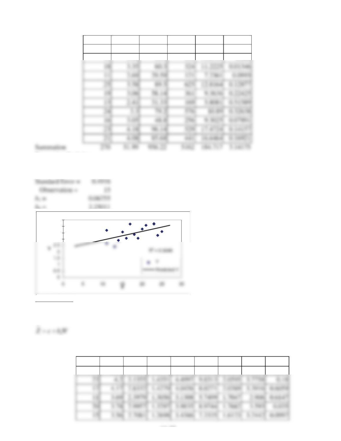
Linear Model:
Yb bX
01
X Y
XiYi Xi2Yi2(Yi^–Yi)2
14 2.89 40.46 196 8.3521 0.09351
6
8
10
12
YYi
13-27
11 3.69 40.59 121 13.6161 0.4856
20 3.78 75.6 400 14.2884 0.03201
15 3.56 53.4 225 12.6736 0.088
Regression Statistics:
R = 0.55217
R Square = 0.30489
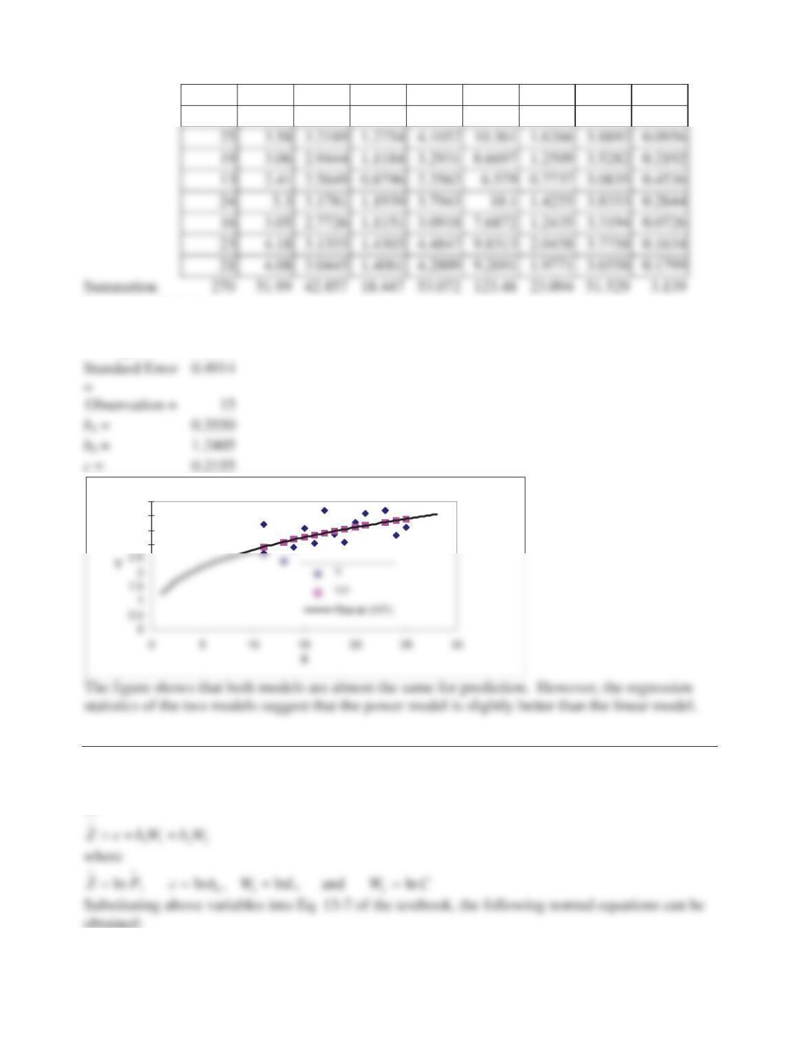
Power Model:
YbX
b
0
1
or
where
ZYcb W X
ln , ln , ln and
0
X Y
W(lnX)Z(lnY) W Z W2Z2Yi
^
(Yi^–Yi)2
14 2.89 2.6391 1.0613 2.8007 6.9646 1.1263 3.1657 0.076
3
3.5
4
4.5
13-28
18 3.35 2.8904 1.209 3.4943 8.3542 1.4616 3.4611 0.0123
11 2.69 2.3979 0.9895 2.3728 5.7499 0.9792 2.906 0.0466
Regression Statistics:
R = 0.5658
R Square = 0.3201
Problem 13-49.
PbLC
bb
0
12
or
3
3.5
4
4.5
13-29
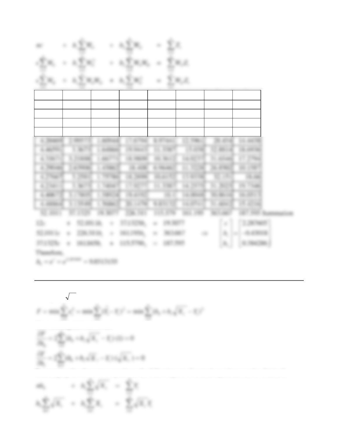
W1(lnL) W2(lnC) Z(lnP) W12 W22W1W2W 12ZW 22Z
4.44265 2.70805 1.41099 19.7372 7.33354 12.0309 27.8489 10.3475
4.38203 2.83321 1.50408 19.2022 8.0271 12.4152 28.8815 12.0734
4.2485 3.29584 1.72277 18.0497 10.8625 14.0023 31.0954 18.7136
4.30407 3.13549 1.62924 18.525 9.83132 13.4954 30.1816 16.0176
Problem 13-50.
Yb bX
01
The resulting derivatives are
Rearranging the above two equations, the following set of normal equations can be obtained:
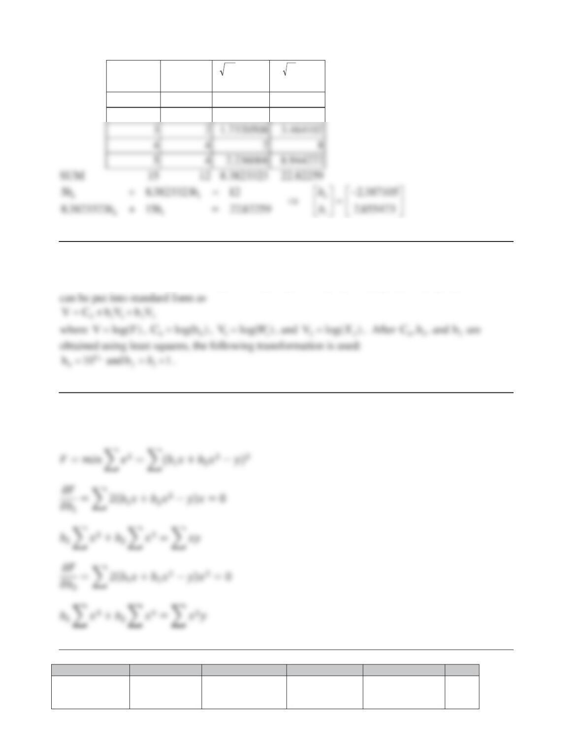
13-30
Xi Yi XiXY
ii
1 1 1 1
2 1 1.4142136 1.414214
Problem 13-51.
Let 1W 11 X and 1b 23 b. Therefore, 3
1
2
b
10 WbY b
X which can be solved as any power
model using multiple regression. Specifically, )log(Xb)log(Wb)log(blog(Y) 23110 , which
Problem 13-52.
ݕොൌܾ
ଵݔܾ
ଶݔଶ
Problem 13-53.
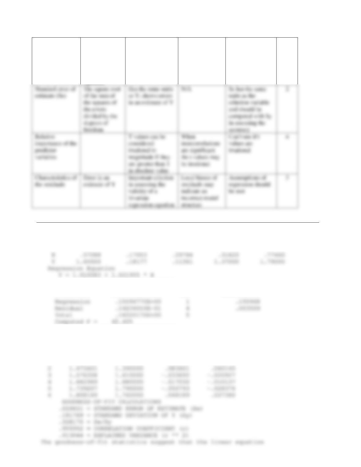
Criteria Indication of Advantages Disadvantages Decision Mode Rank
Rationality of the
coefficients
Whether or not
the coefficients
are applicable
Can give an
accurate answer
Magnitude may
be difficult to
assess
Use if the
coefficients seem
plausible
1
13-31
Coefficient of
multiple
determination
(R^2)
The fraction of
the variation in
the criterion
variable that is
explained by
the regression
equation
Always in the range
of 0 – 1 so it can
indicate that Y is not
related to any of the
predictor variables
Only applies to
linear equations
When close to 0 it
indicates that Y is
not related to any
of the predictor
variables
5
Problem 13-54.
Standard Coeff. of Minimum Maximum
Var Mean deviation variation value value
— ———- ———- ———- ———- ———-
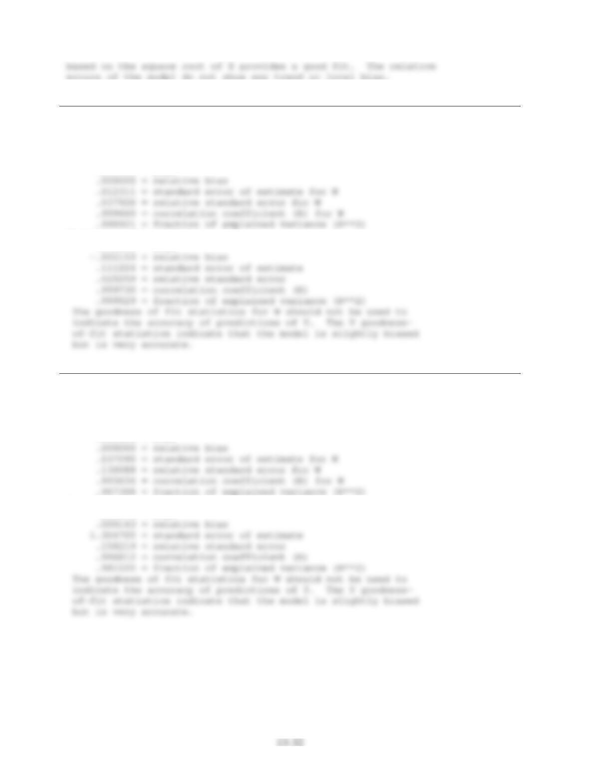
ANALYSIS OF VARIANCE TABLE
Source Sum of squares df Mean square
ANALYSIS OF RESIDUALS
——————————————————-
Predicted Observed Error Relative
I YP Y e = YP – Y Error(e/Y)
— ———- ———- ———- ———-
1 1.339725 1.370000 -.030275 -.022099
Problem 13-55.
.083293 = intercept coefficient
.205179 = slope coefficient
y = 10 ** (0.0833 + 0.205 * X)
Statistics for prediction of W where W = log Y
.000000 = bias
Statistics for prediction of Y
-.013351 = bias
Problem 13-56.
2.652771 = intercept coefficient
.358353 = slope coefficient
Y = e ** (2.653 + 0.358 * X)
Statistics for prediction of W where W = ln Y
.000000 = bias
Statistics for prediction of Y
.004878 = bias