13-1
CHAPTER 13. MULTIPLE AND NONLINEAR REGRESSION
ANALYSIS
Chapter 13. Multiple and Nonlinear Regression Analysis ………………………………………………………..1
13.1. Introduction …………………………………………………………………………………………………………….1
13.2. Correlation Analysis …………………………………………………………………………………………………1
13.3. Multiple Regression Analysis…………………………………………………………………………………….3
13.4 and 13.5. Regression Analysis of Polynomial and Power Models ………………………………….15
The following table provides a summary of the problems with their appropriate sections:
Section Problems
13.1
13.2 1 to 6
13.3 7 to 34
13.4 and 13.5 35 to 56
13.1. Introduction
None
13.2. Correlation Analysis
Problem 13-1.
Temperature
Problem 13-2.
The size of the panel (larger panels produce more power)
13-2
Problem 13-3.
Obstacles
xRocks, if many are present, trash could get trapped
The length of grassland or forestland buffer along the perimeter of the stream
Width of River
Depth of river
Population Density of the area
Problem 13-4.
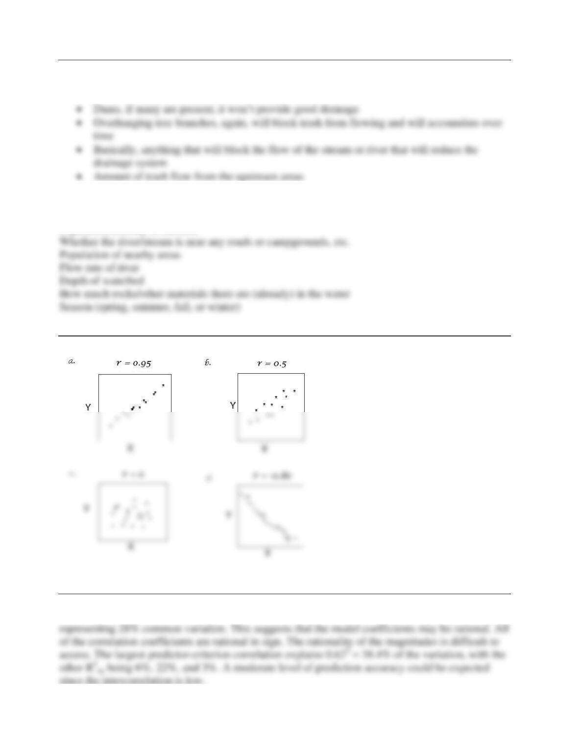
Problem 13-5.
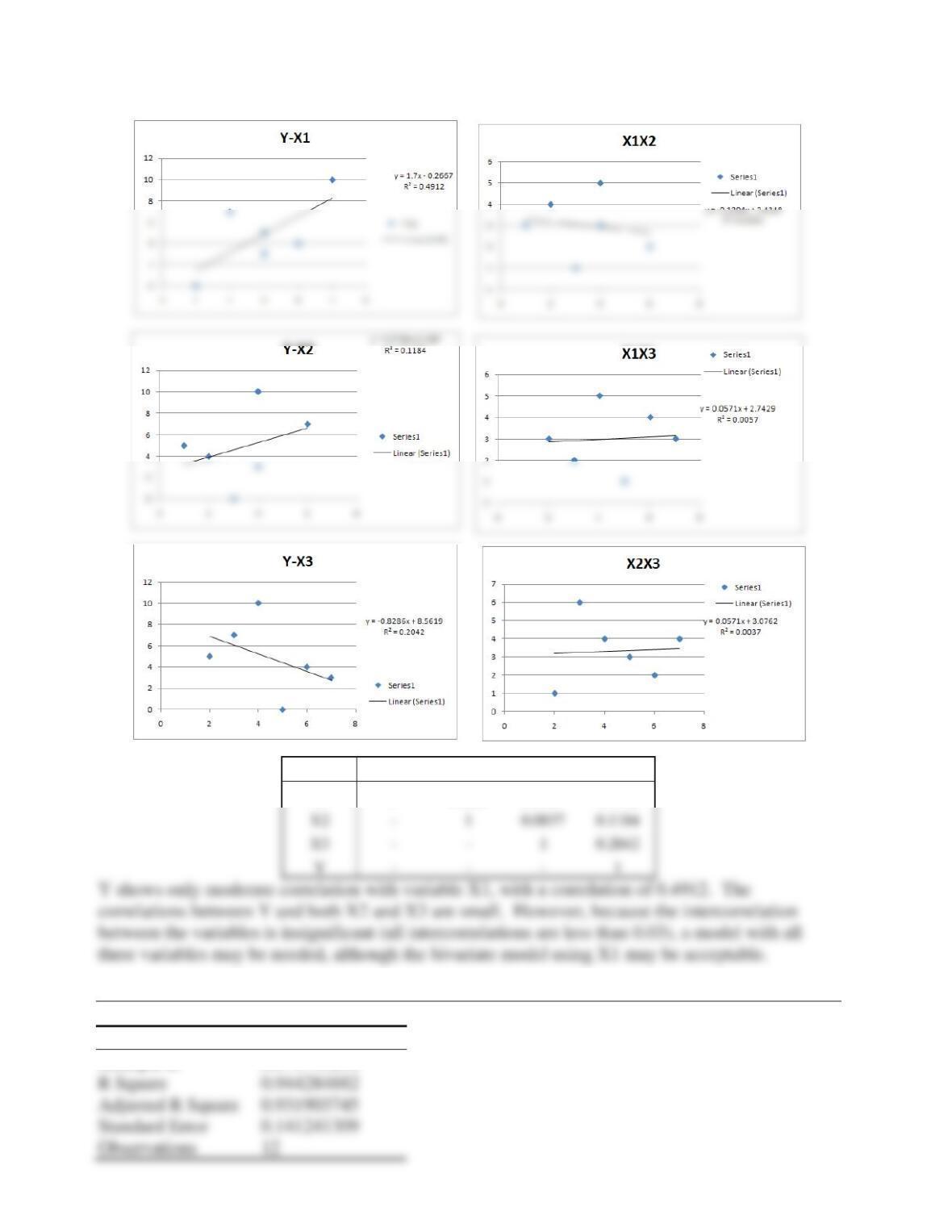
The Intercorrelation between the predictor variables is generally low with the largest (0.53) only
13-3
Problem 13-6.
The prediction-criterion correlations are rational, but the Ryz could be either positive or negative. A
rougher channel would likely have larger particles, which show greater resistance to being eroded.
13.3. Multiple Regression Analysis
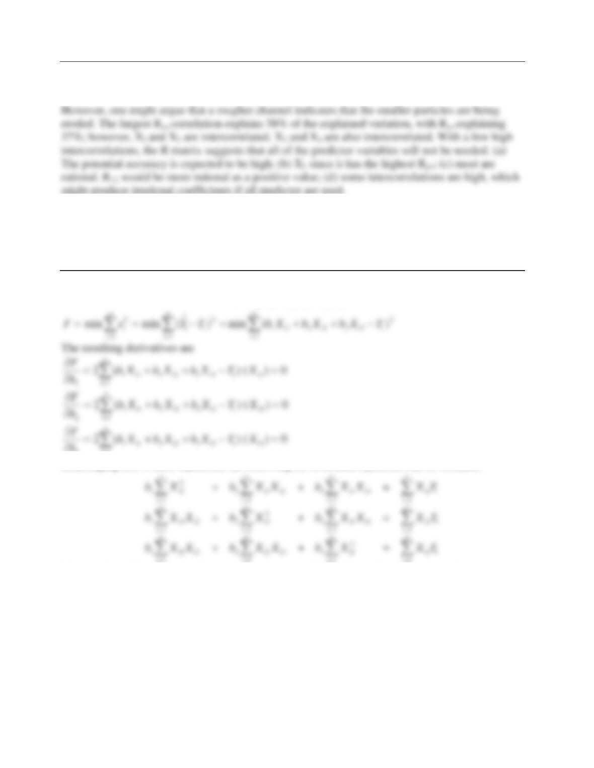
Problem 13-7.
YbX bX bX
11 2 2 33
w
bbX bX bX Y X
3
i=1
Rearranging above three equations, the following set of normal equations can be obtained:
The solution of the three simultaneous equations would yield the values of b1, b2, and b3.
13-4
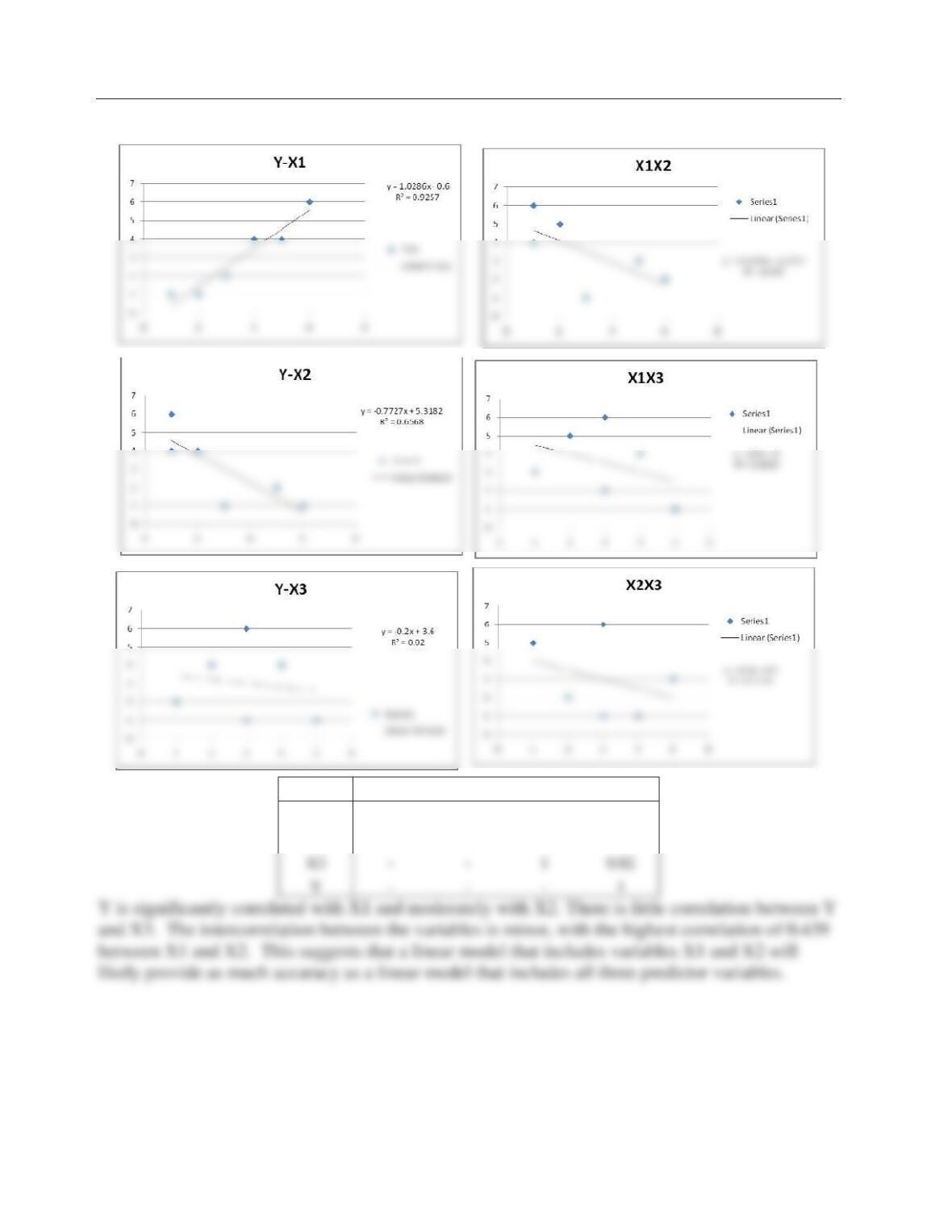
Problem 13-8.
Part (a)
x1 X2 X3 Y
x1 1 0.439 0.1429 0.9257
X2 – 1 0.1136 0.6568
13-5
Part (b)
x1 X2 X3 Y
x1 1 0.0261 0.0057 0.4912
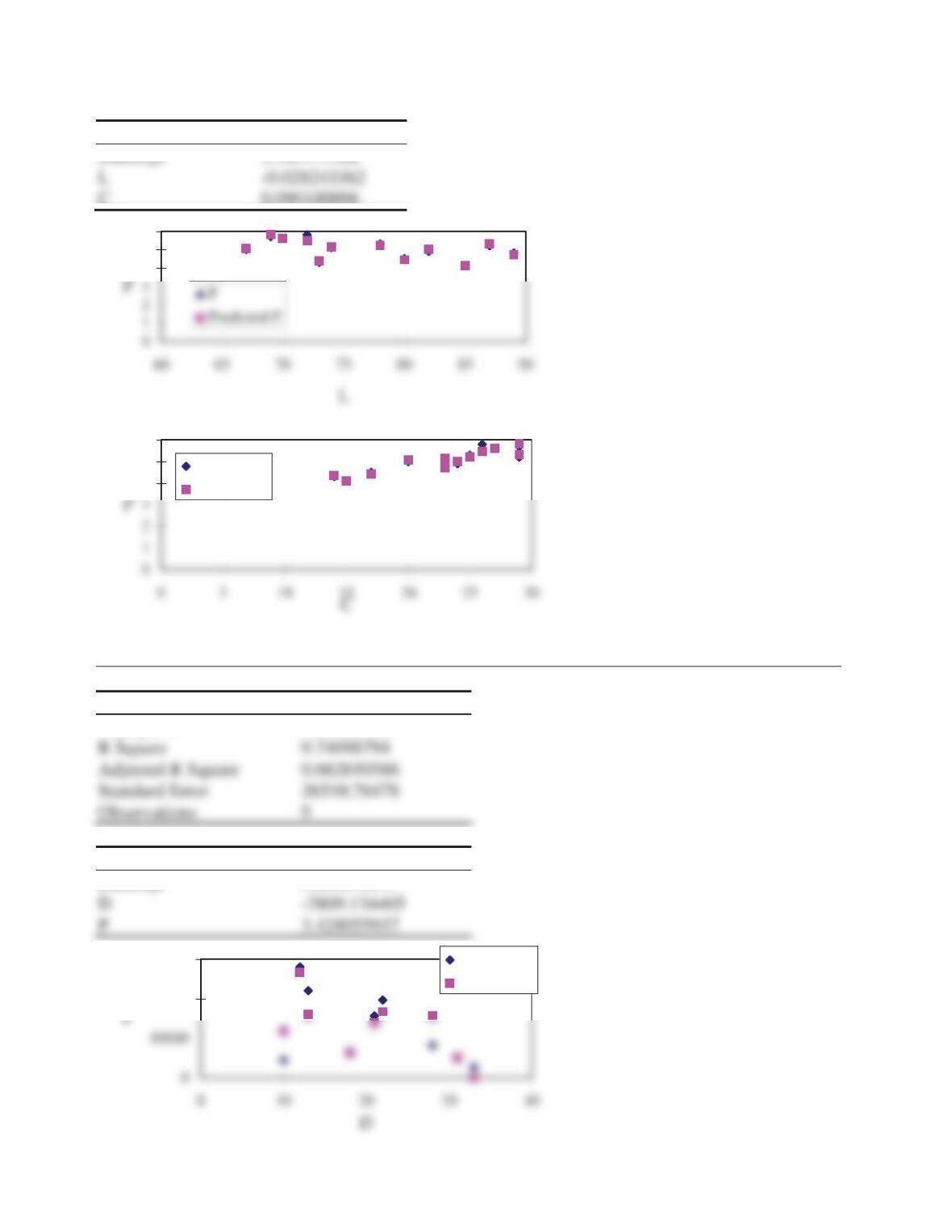
Problem 13-9.
Regression Statistics
Multiple R 0.971743218
13-6
Coefficients
C 0.090100096
4
5
6
4
5
6
P
Predicted P
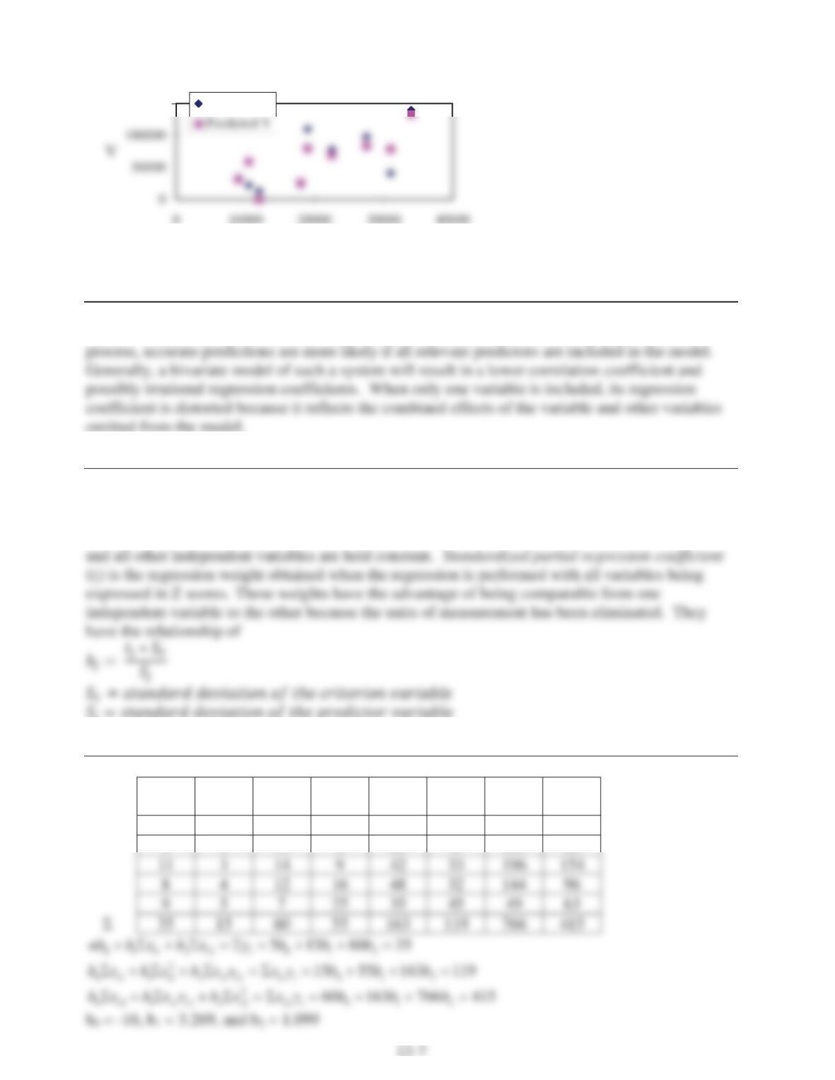
Problem 13-10.
Regression Statistics
Multiple R 0.86428464
Coefficients
Intercept 50896.55597
100000
150000
V
Predicted V
150000
P
V
Problem 13-11.
When a criterion variable Y relates to several predictor variables in an underlying physical
Problem 13-12.
The partial regression coefficient (bj) is also called the regression coefficient, regression weight,
partial regression weight, slope coefficient or partial slope coefficient. It gives the amount by
which the dependent variable increases when one independent variable is increased by one unit
Problem 13-13.
Y X1 X
2 X
1^2 X1*X2X1*Y X2^2 X2*Y
5 1 16 1 16 5 256 80
2 2 11 4 22 4 121 22
Problem 13-14.
i
ii
i
y
y
ppy
s
xx
zand
s
yy
z
ztztztz
2211
…
Problem 13-15.
36 .005 50
37 .040 40
45 .004 45
4000 .0005 1550
Standard Coefficient
Var Mean Deviation of Variation Minimum Maximum
— ———— ———– ———— ———– ———-
1 800.6250000 1353.7910000 1.6909180 36.0000000 4000.0000000
CORRELATION MATRIX
ROW 1 2 3
1 1.000 -.302 .977
Var b t R R**2 t*R
— ———– ——– ——- ——- ——-
OBS PREDICTED OBSERVED RESIDUAL REL ERROR
NO. YP Y e = YP – Y e / Y
— ———— ———– ———– ———-
1 147.3575000 50.0000000 97.3574700 1.94715
2 36.9947400 40.0000000 -3.0052570 -.07513
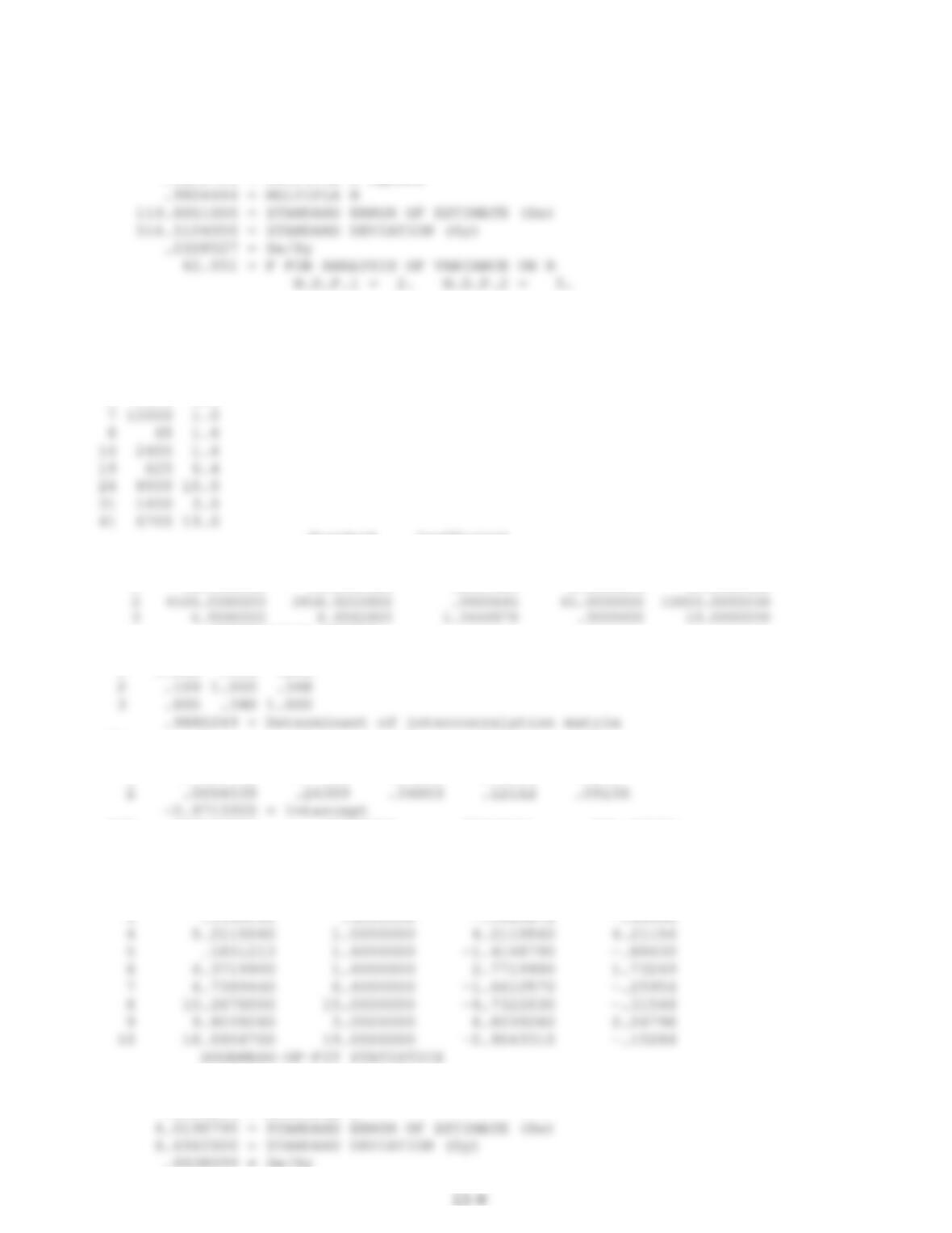
7 578.2756000 650.0000000 -71.7244300 -.11035
8 1596.7640000 1550.0000000 46.7637900 .03017
GOODNESS-OF-FIT STATISTICS
————————–
.9612712 = MULTIPLE R SQUARE
Problem 13-16.
3 1500 1.2
3 3500 0.4
3 4300 0.3
Standard Coefficient
Var Mean Deviation of Variation Minimum Maximum
— ———— ———– ———— ———– ———–
1 15.5000000 13.2182500 .8527905 3.0000000 41.0000000
CORRELATION MATRIX
ROW 1 2 3
1 1.000 .109 .805
Var b t R R**2 t*R
— ———– ——– ——- ——- ——-
1 .3908762 .77622 .80501 .64805 .62487
OBS PREDICTED OBSERVED RESIDUAL REL ERROR
NO. YP Y e = YP – Y e / Y
— ———— ———– ———– ———-
1 -1.1179110 1.2000000 -2.3179110 -1.93159
2 -.2101088 .4000000 -.6101088 -1.52527
————————–
.7164328 = MULTIPLE R SQUARE
.8464236 = MULTIPLE R
.6038099 = Se/Sy
13-10
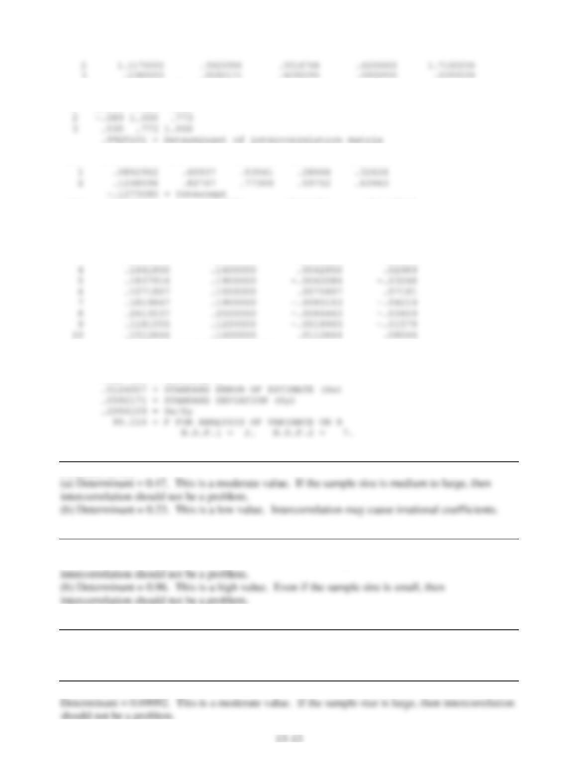
Problem 13-17.
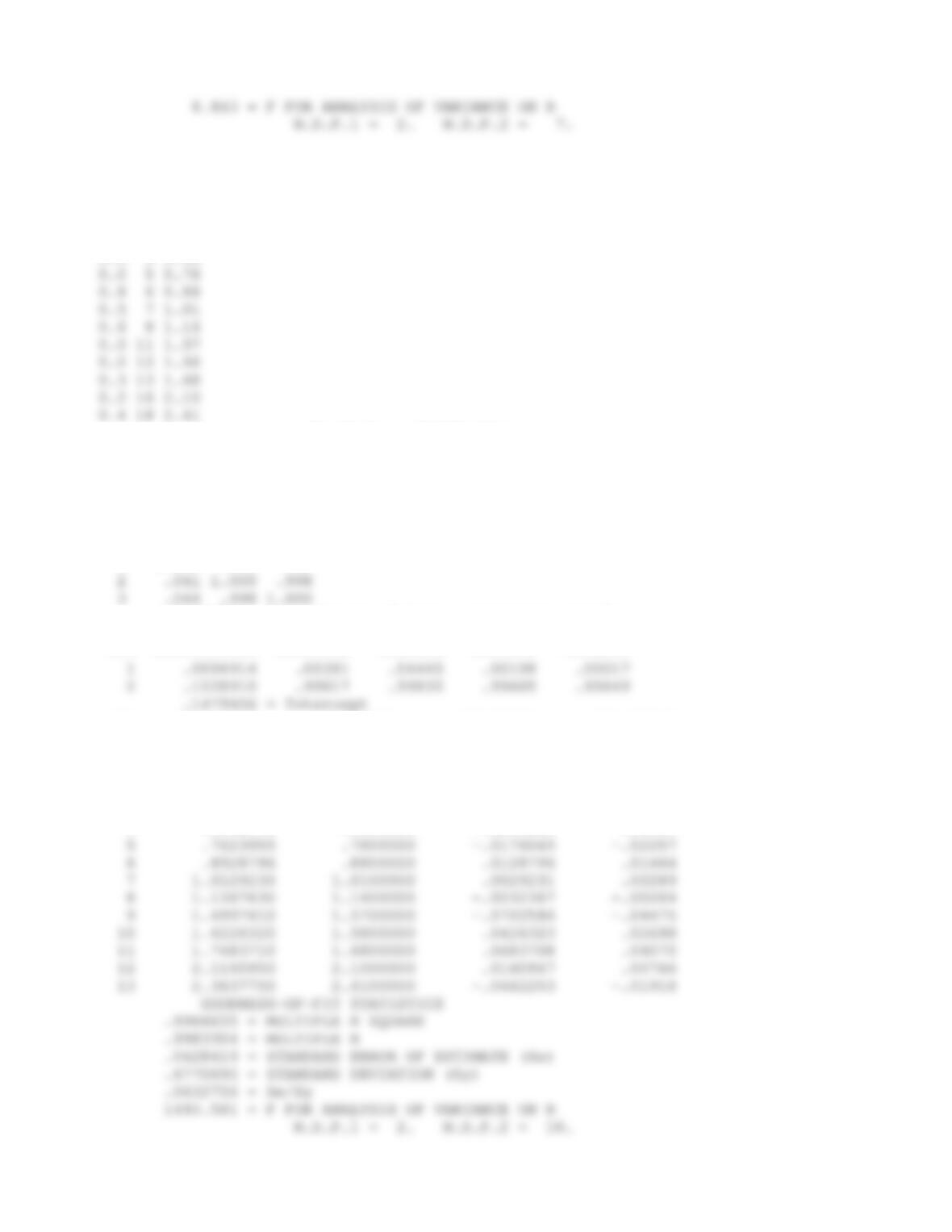
0.0 1 0.24
0.5 2 0.44
0.2 3 0.49
0.0 3 0.54
Standard Coefficient
Var Mean Deviation of Variation Minimum Maximum
— ———— ———– ———— ———– ———–
1 .2692308 .2719823 1.0102200 .0000000 .8000000
2 8.0769230 5.4994170 .6808802 1.0000000 18.0000000
3 1.1430770 .6770695 .5923219 .2400000 2.4100000
CORRELATION MATRIX
ROW 1 2 3
1 1.000 .041 .044
.9983423 = Determinant of intercorrelation matrix
Var b t R R**2 t*R
OBS PREDICTED OBSERVED RESIDUAL REL ERROR
NO. YP Y e = YP – Y e / Y
— ———— ———– ———– ———-
1 .2708316 .2400000 .0308316 .12846
2 .3984682 .4400000 -.0415318 -.09439
3 .5185118 .4900000 .0285118 .05819
4 .5166135 .5400000 -.0233865 -.04331
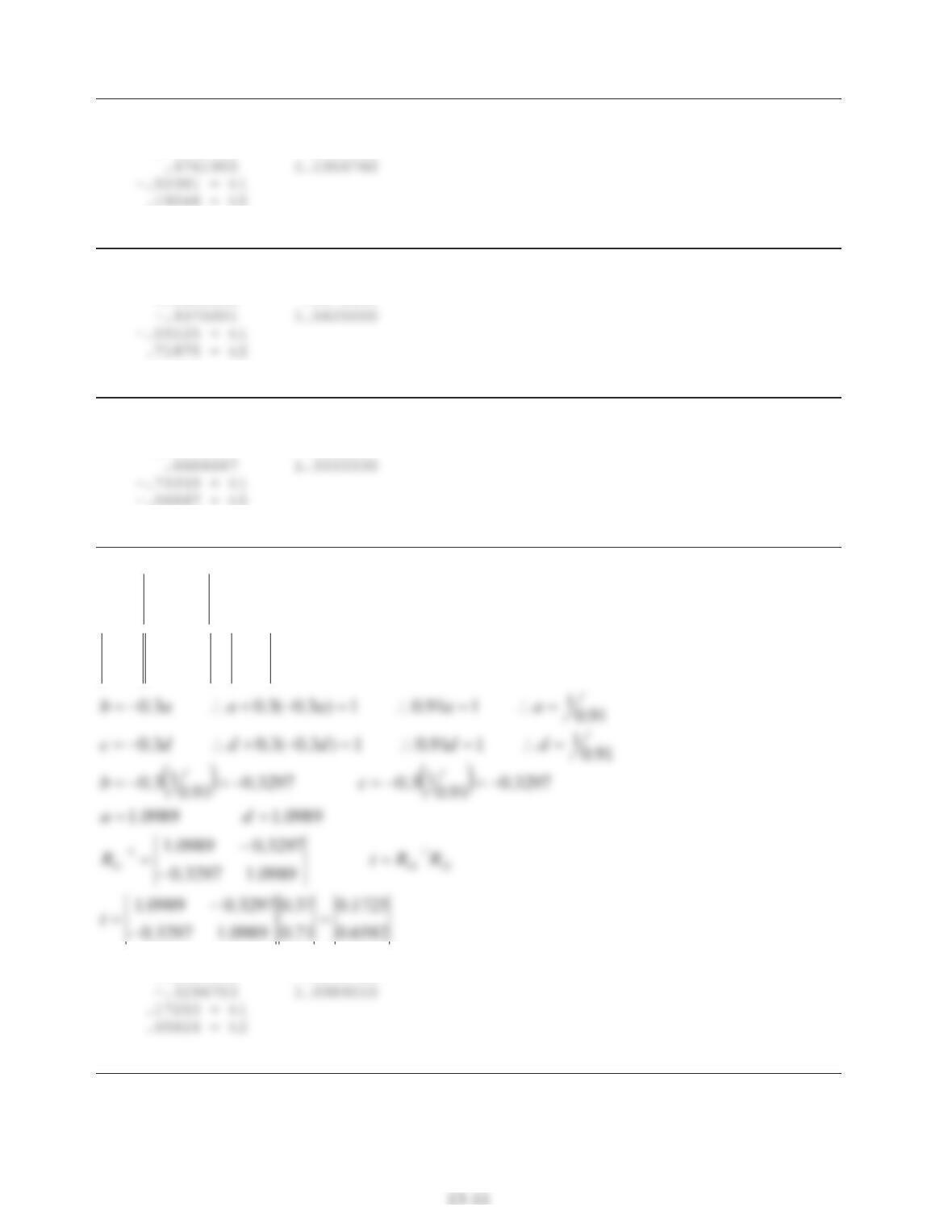
Problem 13-18.
Inverse matrix
1.1904760 .4761905
Problem 13-19.
Inverse matrix
1.5625000 -.9375001
Problem 13-20.
Inverse matrix
1.3333330 .6666667
Problem 13-21.
13.0
03.0
03.0
13.0
10
01
13.0
3.01
13.0
3.01
11
1
1111
?
?
dc
ba
dc
ba
dc
ba
IRRR
Inverse matrix
1.0989010 -.3296703
Problem 13-22.
Standard Coefficient
Var Mean Deviation of Variation Minimum Maximum
— ———— ———– ———— ———– ———–
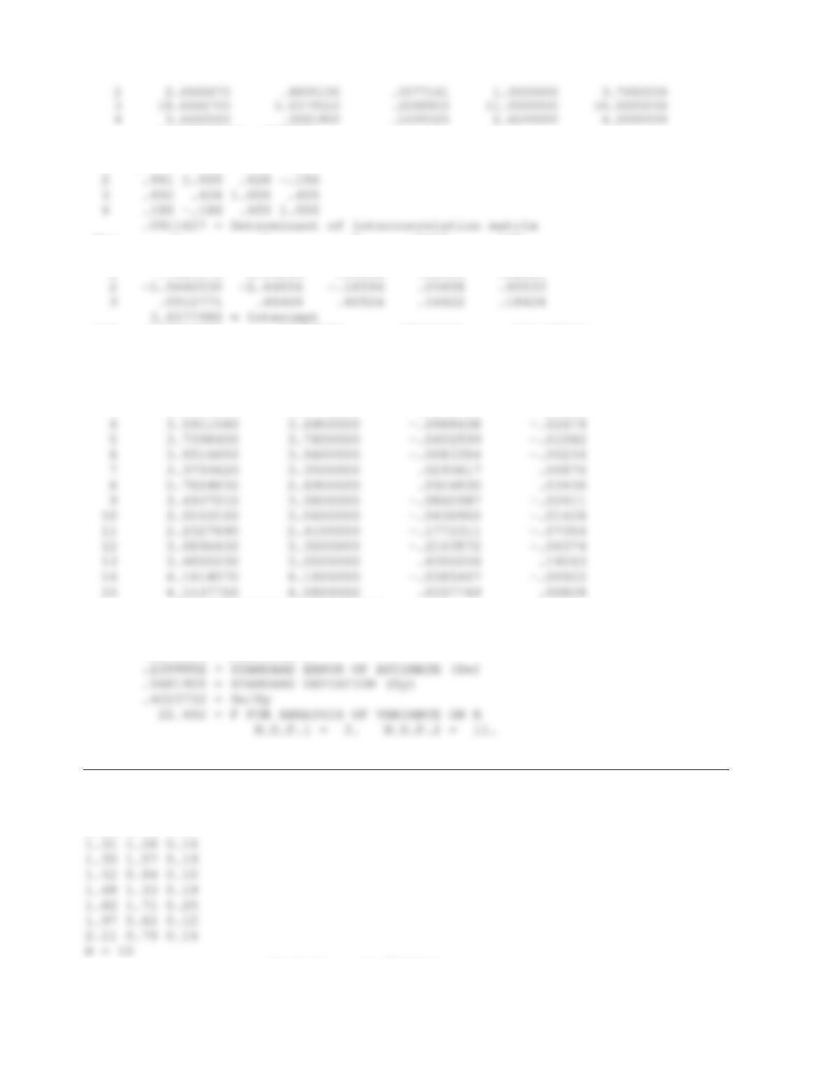
1 3.6600000 1.6685320 .4558832 1.4000000 6.9000000
13-12
CORRELATION MATRIX
ROW 1 2 3 4
1 1.000 .941 .452 .100
Var b t R R**2 t*R
— ———– ——– ——- ——- ——-
1 .7487175 2.19866 .10018 .01004 .22025
OBS PREDICTED OBSERVED RESIDUAL REL ERROR
NO. YP Y e = YP – Y e / Y
— ———— ———– ———– ———-
1 3.3906140 2.8900000 .5006142 .17322
2 4.0767240 4.2000000 -.1232758 -.02935
3 3.9054810 4.1700000 -.2645195 -.06343
GOODNESS-OF-FIT STATISTICS
————————–
.8598293 = MULTIPLE R SQUARE
.9272698 = MULTIPLE R
Problem 13-23.
0.83 0.68 0.04
0.95 1.43 0.11
1.22 0.92 0.10
Standard Coefficient
Var Mean Deviation of Variation Minimum Maximum
— ———— ———– ———— ———– ———–
1 1.4760000 .4230629 .2866280 .8300000 2.1100000
CORRELATION MATRIX
ROW 1 2 3
1 1.000 -.089 .535
Var b t R R**2 t*R
— ———– ——– ——- ——- ——-
OBS PREDICTED OBSERVED RESIDUAL REL ERROR
NO. YP Y e = YP – Y e / Y
— ———— ———– ———– ———-
1 .0283575 .0400000 -.0116425 -.29106
2 .1322001 .1100000 .0222001 .20182
3 .0915770 .1000000 -.0084230 -.08423
GOODNESS-OF-FIT STATISTICS
————————–
.9658921 = MULTIPLE R SQUARE
.9827981 = MULTIPLE R
Problem 13-24.
Problem 13-25.
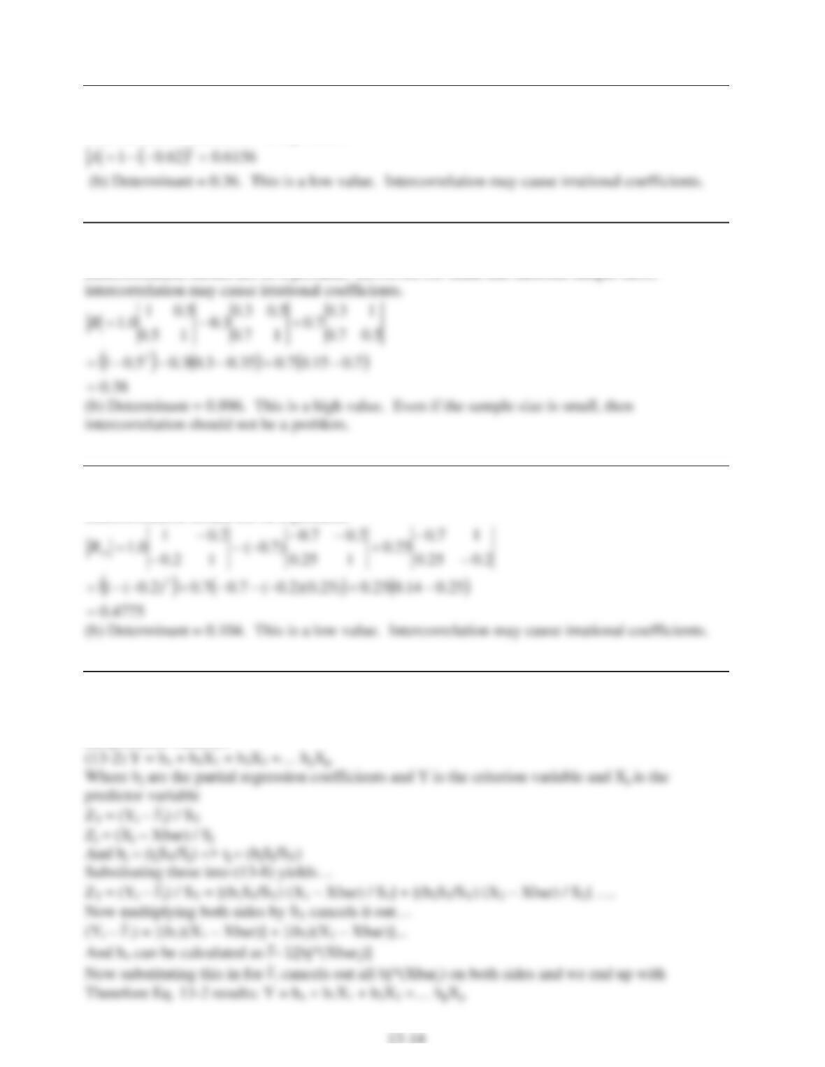
(a) Determinant = 0.92. This is a high value. Even if the sample size is small, then
Problem 13-26.
Determinant = 0.12868. This is a low value. Intercorrelation may cause irrational coefficients.
Problem 13-27.
Problem 13-28.
(a) Determinant = 0.6156. This is a moderate value. If the sample size is large, then
intercorrelation should not be a problem.
Problem 13-29.
(a) Determinant = 0.38. This is a low to moderate value. If the sample size is large, then
intercorrelation should not be a problem. However, for small and medium sample sizes,
Problem 13-30.
(a) Determinant = 0.4775. This is a moderate value. If the sample size is medium to large, then
intercorrelation should not be a problem.
Problem 13-31.
Starting with Eq. 13-8: ZY = t1Z1 + t2Z2 +…+ tpZp
In which tj is a standardized partial regression coefficient and ZY is the criterion variable and Zj are
the predictor variables
Problem 13-32.
ݕൌܾܾ݊
ଵݔଵܾ
ଶݔଶܾ
ଷݔଵݔଶ
Problem 13-33.
R is standardized so it can be compared with values from other analyses. It can be misleading if
Problem 13-34.
The Se has the advantage that it is expressed in the units of the criterion variable, so that a value
13.4 and 13.5. Regression Analysis of Polynomial and Power Models
Problem 13-35.
¦ 2
22
5.0
11 )/( YXbXbF
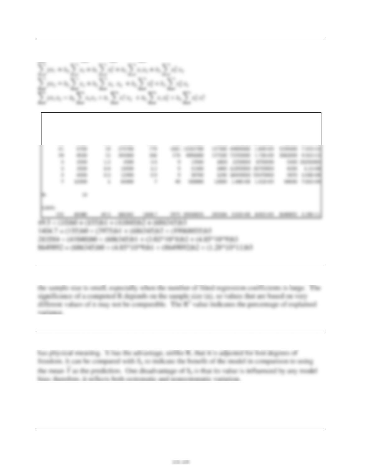
A(X1) Z(X2) Y X1X2 YX1 X1^2 X1^2X2 YX2 X2^2 X1X2^2 YX1X2 X1^2X2^2
8 65 1.6 520 12.8 64 4160 104 4225 33800 832 270400
19 625 6.4 11875 121.6 361 225625 4000 390625 7421875 76000 1.41E+08
31 1450 3 44950 93 961 1393450 4350 2102500 65177500 134850 2.02E+09
16 2400 1.6 38400 25.6 256 614400 3840 5760000 92160000 61440 1.47E+09
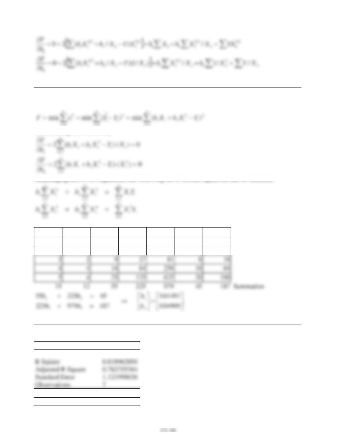
Problem 13-36.
YbXbX
12
2
i=1
i=1
i=1
The resulting derivatives are
X Y X2 X3 X4X Y X2 Y
1 1 1 1111
2 1 4 8 16 2 4
Problem 13-37.
A linear model was developed in Problem 12-71 as follows:
Regression Statistics
Multiple R 0.904965637
Coefficients
Intercept 3.75063049