Civil Engineering Chapter 12 Homework The correlation coefficient would reflect the statistical

CHAPTER 12. REGRESSION ANALYSIS

Chapter 12. Regression Analysis ………………………….……………………………………………………………….1

12.1. Introduction ……………………………………………………………………………………………..……………..1

12.2. Correlation Analysis …………………………………………………………………………………………………1

12.3. Introduction to Regression ………………………………………………………………………………………17

12.4. Principle of Least Squares ……………………………………………………………………………………….19

The following table provides a summary of the problems with their appropriate sections:

Section Problems

12.1 None

12.2 1 to 38

12.3 38 to 42

12.4 43 to 46

12.1. Introduction

None

12.2. Correlation Analysis

Problem 12-1.

The correlation coefficient would reflect the statistical relationship between chewing gum sales

and bank robberies. If it were a positive number close to 1, it would show that as chewing gum

12-2

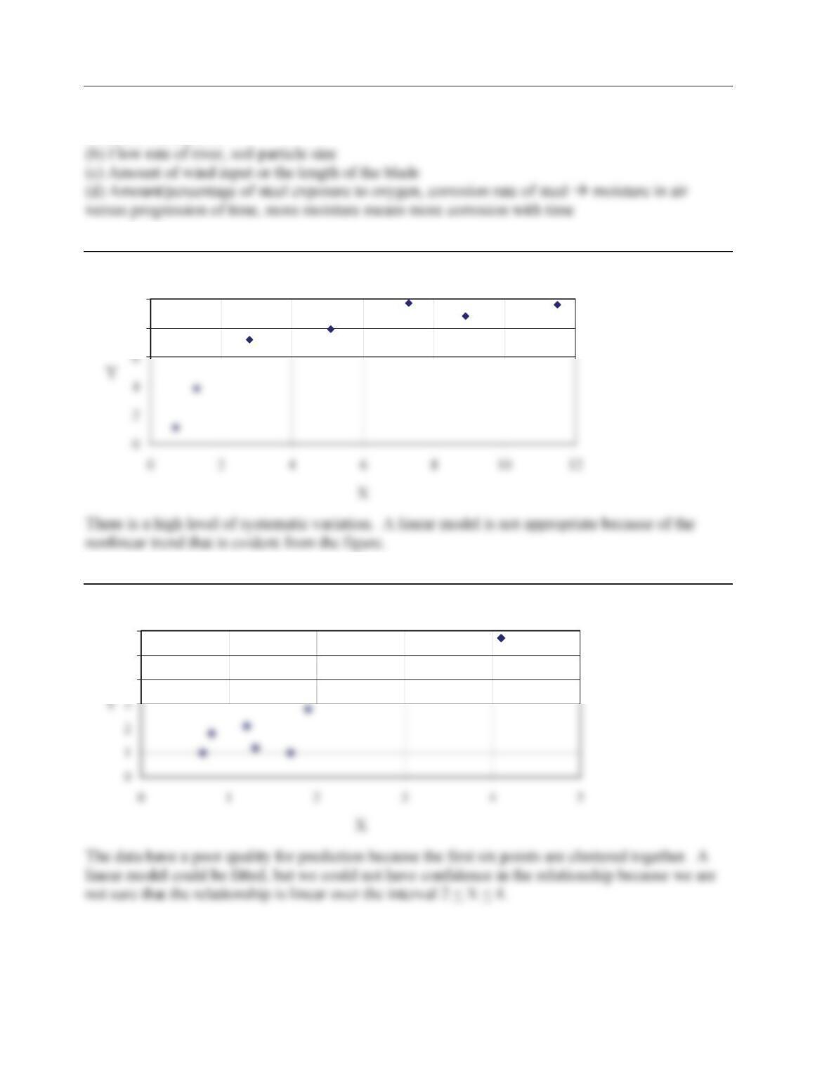
Problem 12-2.

(a) Friction within the pump, the efficiency of a hydraulic pump Æ flow and power, the more

flow, the more power

Problem 12-3.

8

10

Problem 12-4.

4

5

6

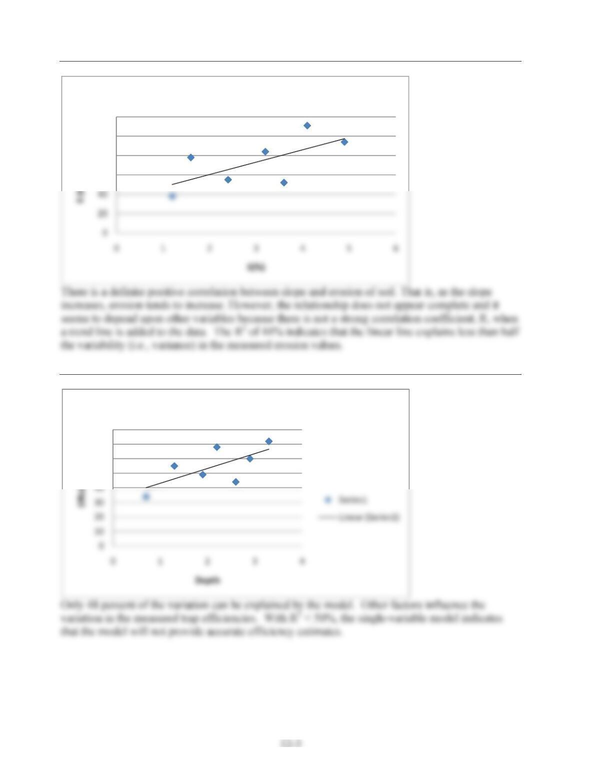
Problem 12-5.

Problem 12-6.

y=12.811x+34.711

R²=0.44

60

80

100

120

SoilSlopeErosion

R²=0.4821

50

60

70

80

Depthvs.Efficiency

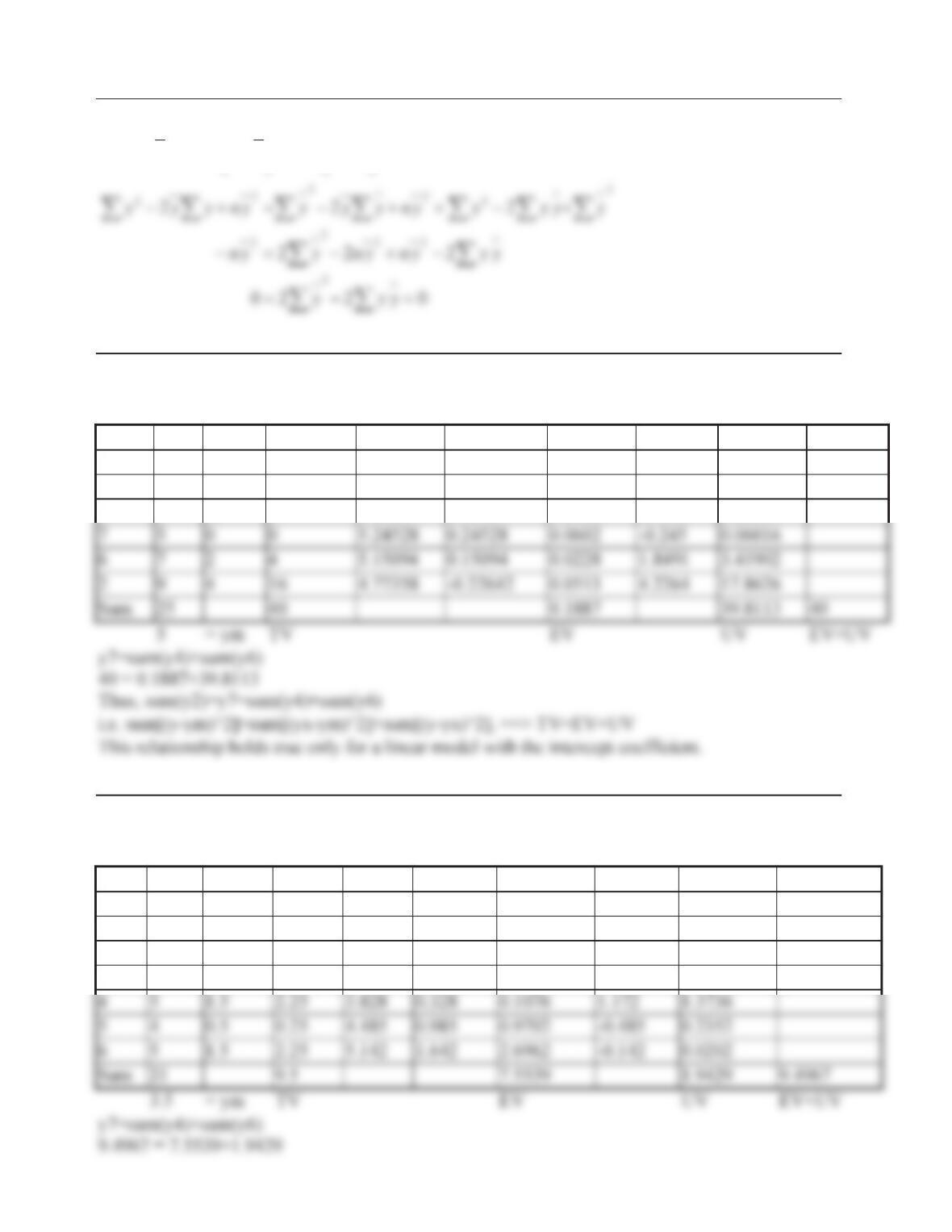
12-4

Problem 12-7.



22

2

¸

·

¨

§

¸

·

¨

§ 

¦¦¦



yyyyyy

Problem 12-8.

ym = y_mean

yx=4.5849+0.09434x

y-ym y1^2 yx-ym y3^2 y-yx y5^2

x y y1 y2 yx y3 y4 y5 y6 y7

2 1 -4 16 4.77358 -0.22642 0.0513 -3.774 14.2399

5 3 -2 4 5.0566 0.0566 0.0032 -2.057 4.2296

Problem 12-9.

ym = y_mean

yx = 1.2 + 0.657 x

y-ym y1^2 yx-ym y3^2 y-yx y5^2

x y y1 y2 yx y3 y4 y5 y6 y7

1 2 -1.5 2.25 1.857 -1.643 2.6994 0.143 0.0204

2 2 -1.5 2.25 2.514 -0.986 0.9722 -0.514 0.2642

3 3 -0.5 0.25 3.171 -0.329 0.1082 -0.171 0.0292

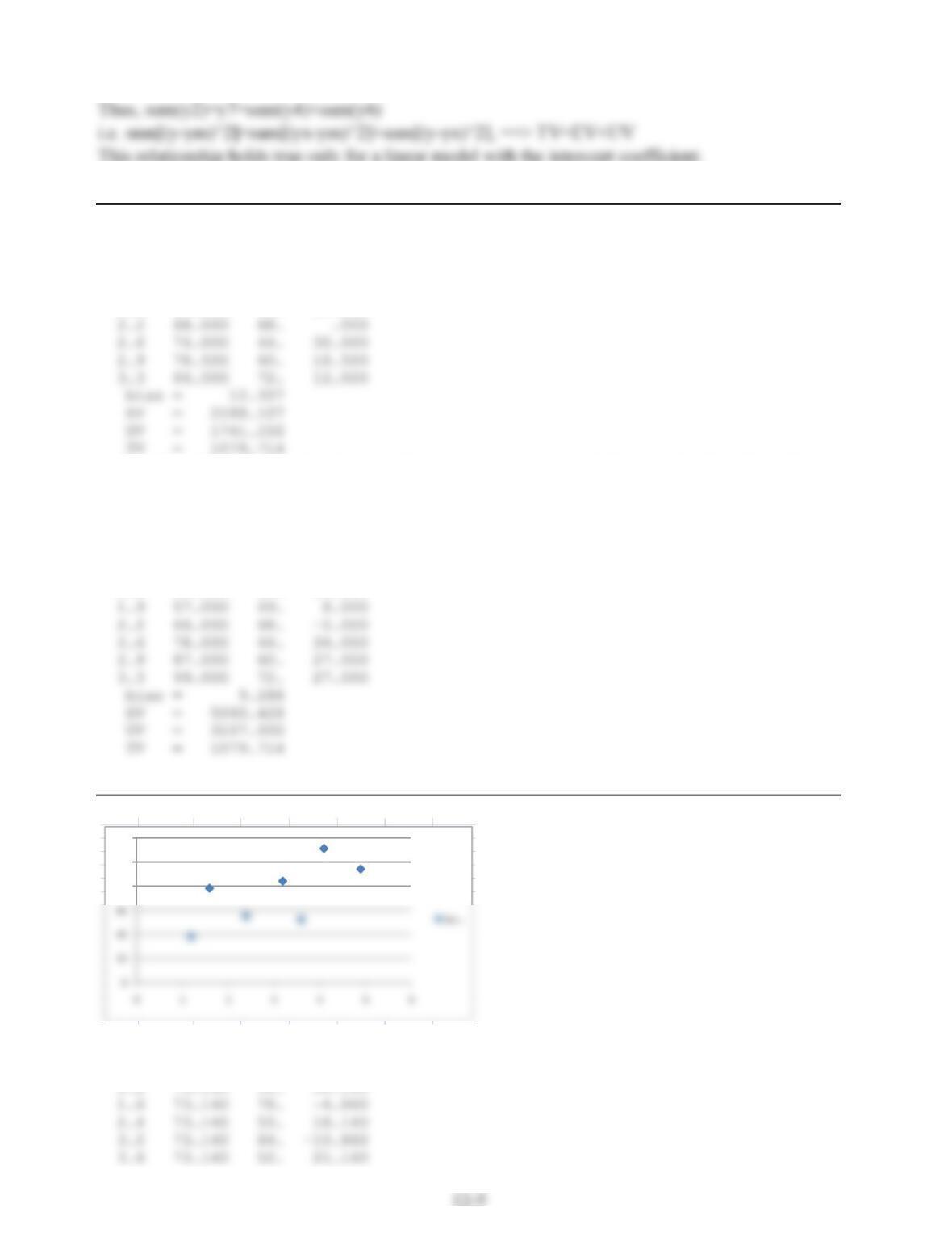
Problem 12-10.

Part (a)

X Y pred Y error

.7 45.500 34. 11.500

1.3 54.500 55. -.500

1.9 63.500 49. 14.500

Part(b) The separation is not linear because the model is biased. Therefore,

EV + UV is not equal to TV. Thus, it would not be appropriate to

compute a correlation coefficient.

Part (c) Bias inflates the unexplained and explained variances.

Part (d)

X Y pred Y error

.7 21.000 34. -13.000

1.3 39.000 55. -16.000

Problem 12-11.

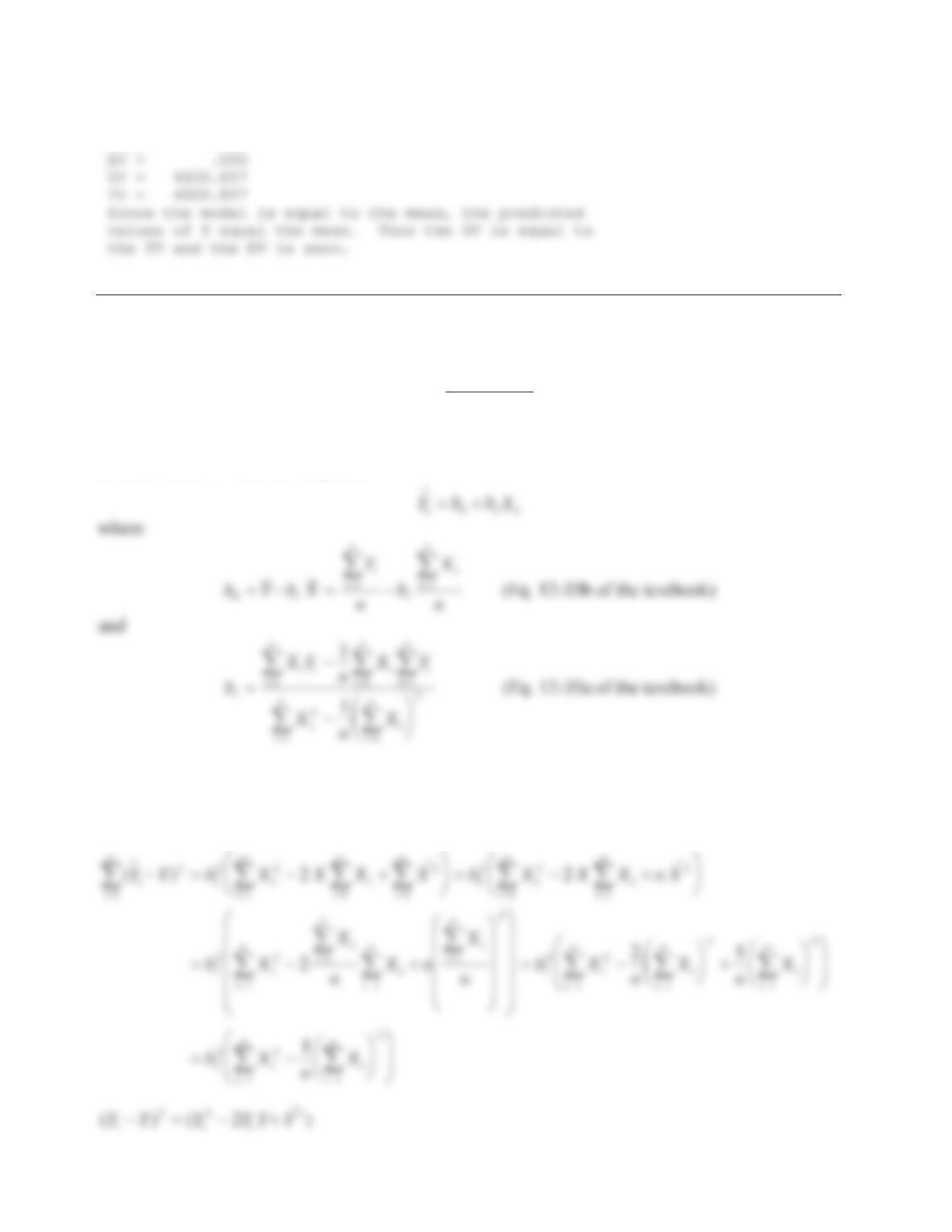
Y mean = 73.1429

Y std dev = 25.8871

X Y pred Y error

80

100

120

12-6

4.1 73.140 111. -37.860

4.9 73.140 94. -20.860

bias = -.000

Problem 12-12.

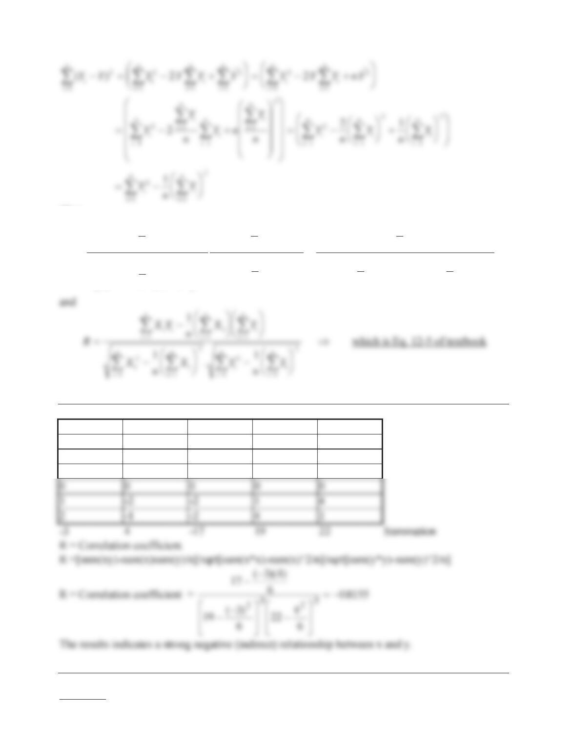
Starting with Eq. 12-4 as given by

R

YY

n

2





¦

()

_

i

i=1

i

i=1

a linear model of Yi



is developed as

____________________________

YY YbX bX Y bX X

iii

    

__ _ _ _

() ()

111

() ( )

__

_

YY bX XXX

ii

2

i

  

2

1

22

2

12-7

Thus,

R

XY nXY

XnX

YnY

XY nXY

XnXY

nnn

nn

nnn

nn

2

22

2

1



§

©

¨·

¹

¸

§

©

¨·

¹

¸

§

©

¨

·

¹

¸

§

©

¨·

¹

¸

§

©

¨·

¹

¸



§

©

¨·

¹

¸

§

©

¨·

¹

¸

¦¦¦

¦¦

¦¦¦

¦¦

i

i=1

ii

i=1

i

i=1

i

2

i=1

i

i=1

i

2

i=1

i

i=1

i

2

i=1

i

i=1

i

i=1

ii

i=1

i

i=1

i

2

i=1

i

i=1

i

2

i=1

i

i=1

nn

nY

¦¦

§

©

¨·

¹

¸

12

Problem 12-13.

x y xy x^2 y^2

-3 2 -6 9 4

-2 2 -4 4 4

-1 3 -3 1 9

Problem 12-14.

Method 1:

12-8

x y xy x^2 y^2

2 1 2 4 1

5 3 15 25 9

Method 2:

X Y ZXXS

X

()/ ZYYS

YY

()/ ZXZY

2 1 -1.1656 -1.4144 1.6487

Sums:

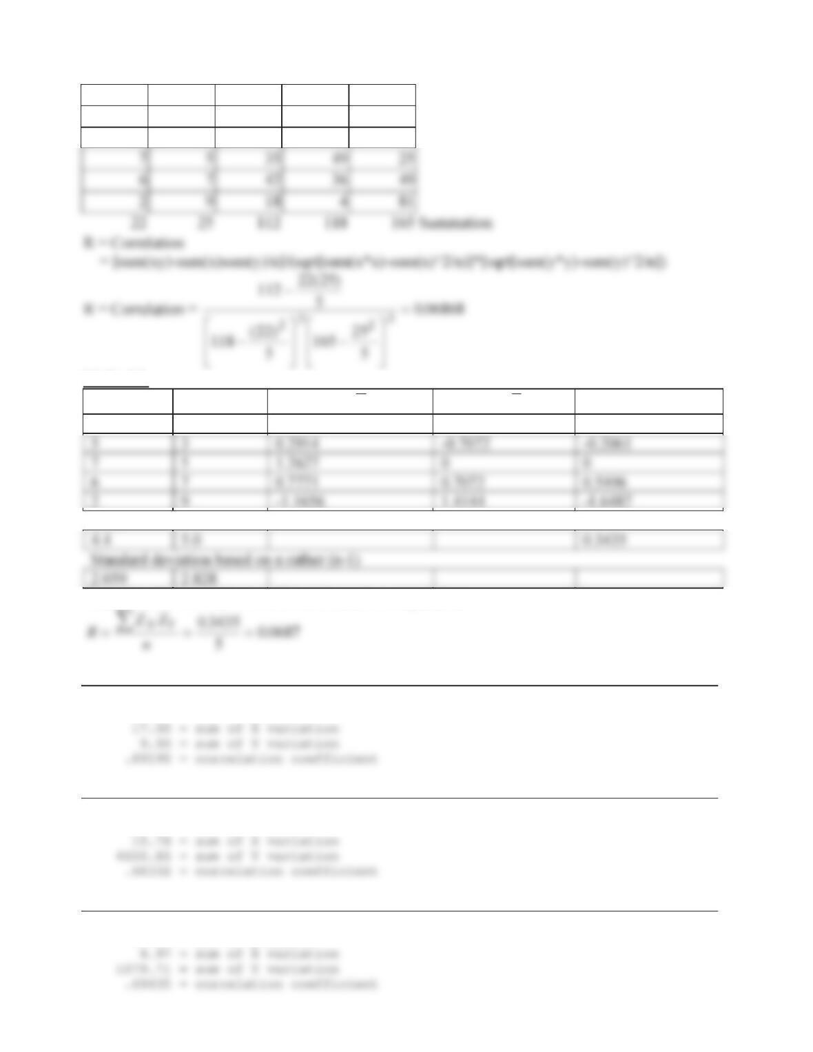
Therefore, the correlation coefficient R can be computed as

Problem 12-15.

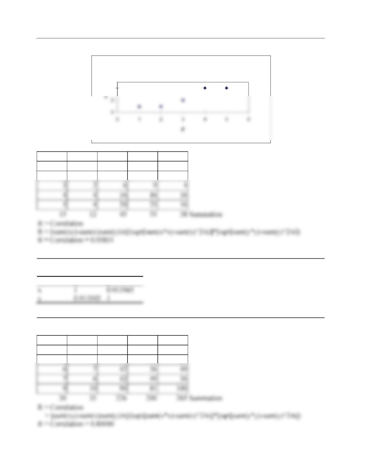
11.50 = sum of products

Problem 12-16.

138.10 = sum of products

Problem 12-17.

50.89 = sum of products

12-9

Problem 12-18.

a.

b.

x y xy x^2 y^2

1 1 1 1 1

2 1 2 4 1

Problem 12-19.

The correlation matrix is given by

x y

Problem 12-20.

a.

x y xy x^2 y^2

3 4 12 9 16

5 8 40 25 64

b.

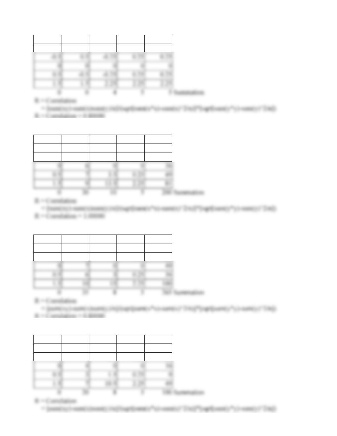
Graph of X versus Y

4

12-10

ZXZYZX.ZYZX^2 ZY^2

-1.5 -1.5 2.25 2.25 2.25

R = Correlation = 0.80000

c.

ZXX ZX.XZX^2 X^2

-1.5 3 -4.5 2.25 9

-0.5 5 -2.5 0.25 25

d.

ZXY ZX.YZX^2 Y^2

-1.5 4 -6 2.25 16

-0.5 8 -4 0.25 64

R = Correlation = 0.80000

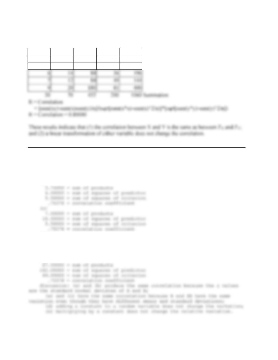
e.

ZXY-3ZX.(Y-3) ZX^2 (Y-3)^2

-1.5 1 -1.5 2.25 1

-0.5 5 -2.5 0.25 25

12-11

R = Correlation = 0.80000

f.

X2Y X(2Y)X^2 (2Y)^2

3 8 24 9 64

5 16 80 25 256

Problem 12-21.

(a)

22.50000 = sum of products

18.00000 = sum of squares of predictor

49.50000 = sum of squares of criterion

.75378 = correlation coefficient

(b)

(d)

22.50000 = sum of products

18.00000 = sum of squares of predictor

49.50000 = sum of squares of criterion

.75378 = correlation coefficient

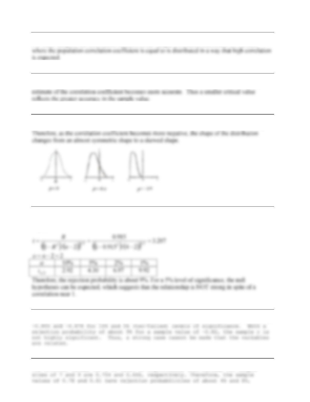
(e)

12-12

Problem 12-22.

For small samples, the distribution function of the sample correlation coefficient for the case

Problem 12-23.

As the sample size increases, the spread of the sampling distribution becomes narrower as the

Problem 12-24.

The center of the sampling distribution is at the population value of the correlation coefficient U.

Problem 12-25.

0:

z

H

A

o

U

Problem 12-26.

For a sample size of 5, there are 3 degrees of freedom, with critical values of

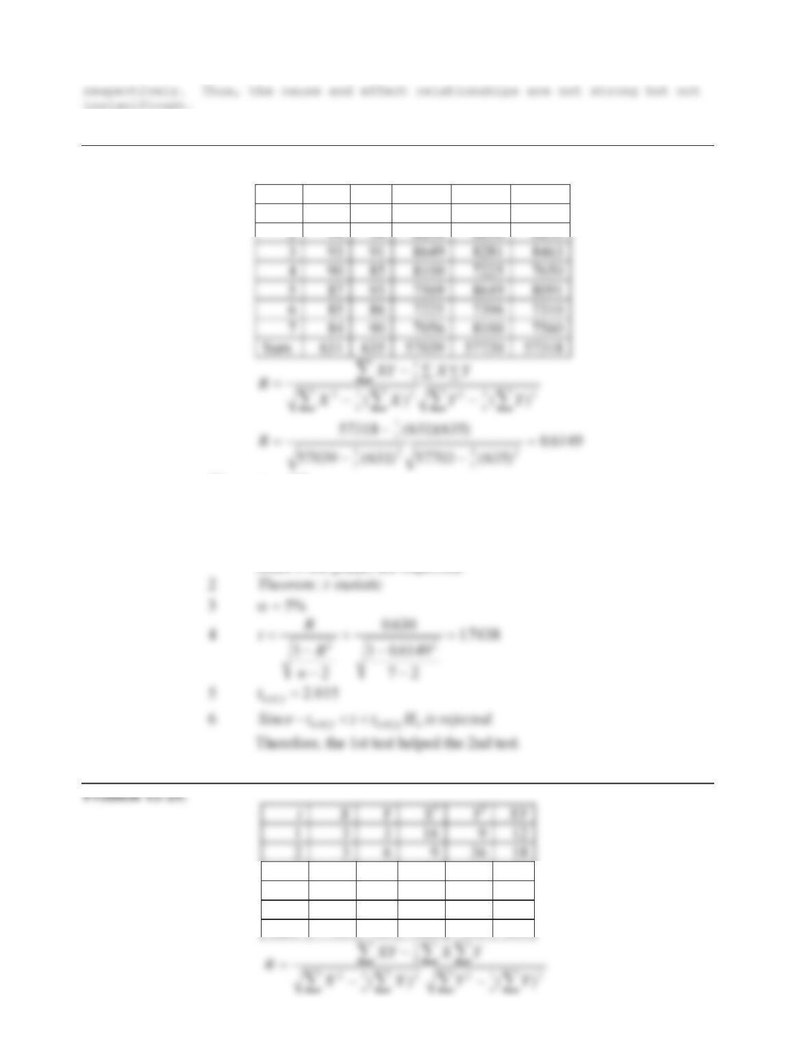
Problem 12-27.

The critical values for a 5% level of significance (two-tailed) for sample

12-13

Problem 12-28.

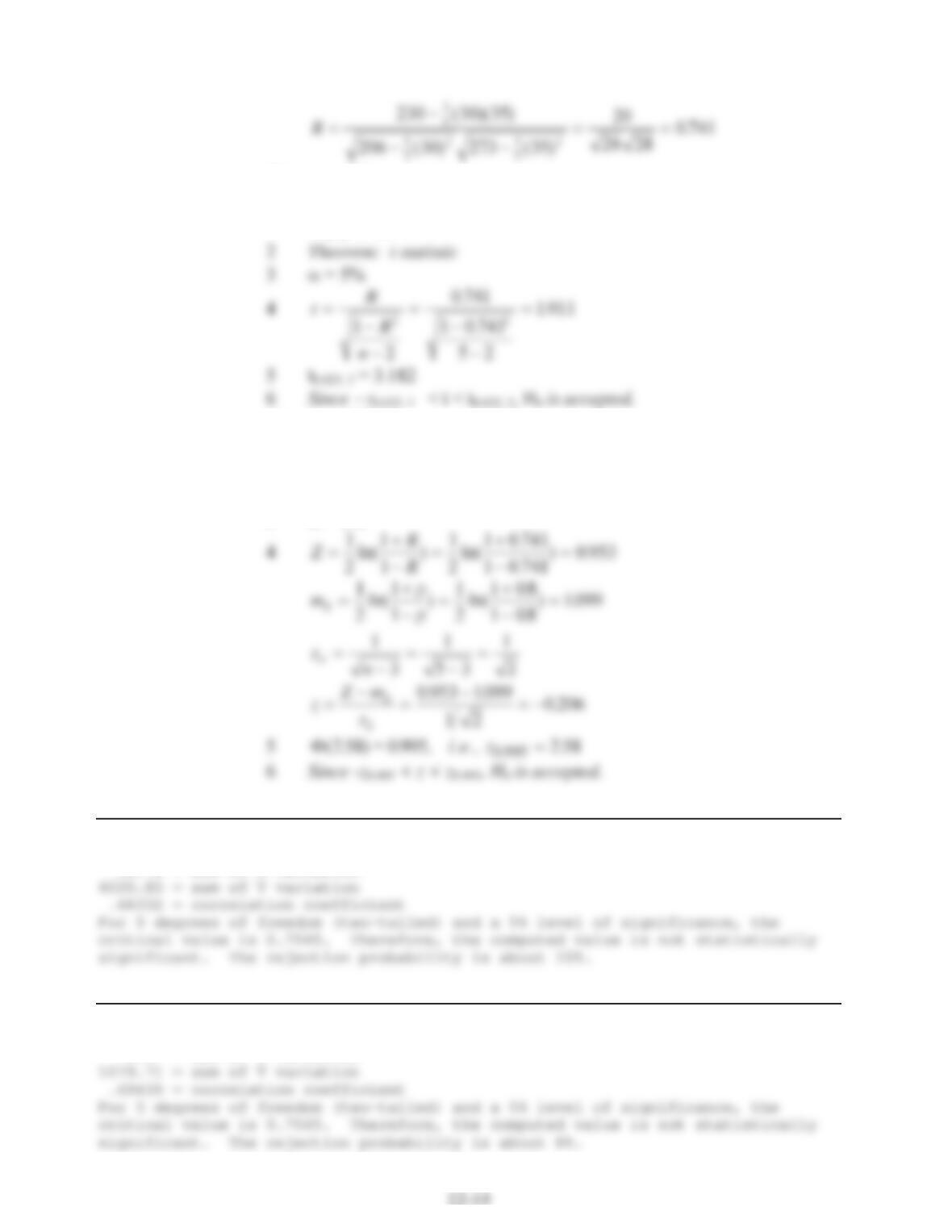
(a)Calculate the correlation coefficient

i X Y X2Y2XY

1 98 96 9604 9216 9408

(b) U000 .

1

H000:.U

0.0: !

U

A

H

Use this alternate hypothesis because a positive correlation should

result if the grades are improved.

(a) 3 9 8 81 64 72

4 68366448

5 8 10 64 100 80

Sum 30 35 206 273 230

(b) U000 .

1

H000:.U

HA:.Uz00

(c) U008 .

1

H008:.U 

HA:.Uz08

2 Theorem : z statistic

3 D = 1%

Problem 12-30.

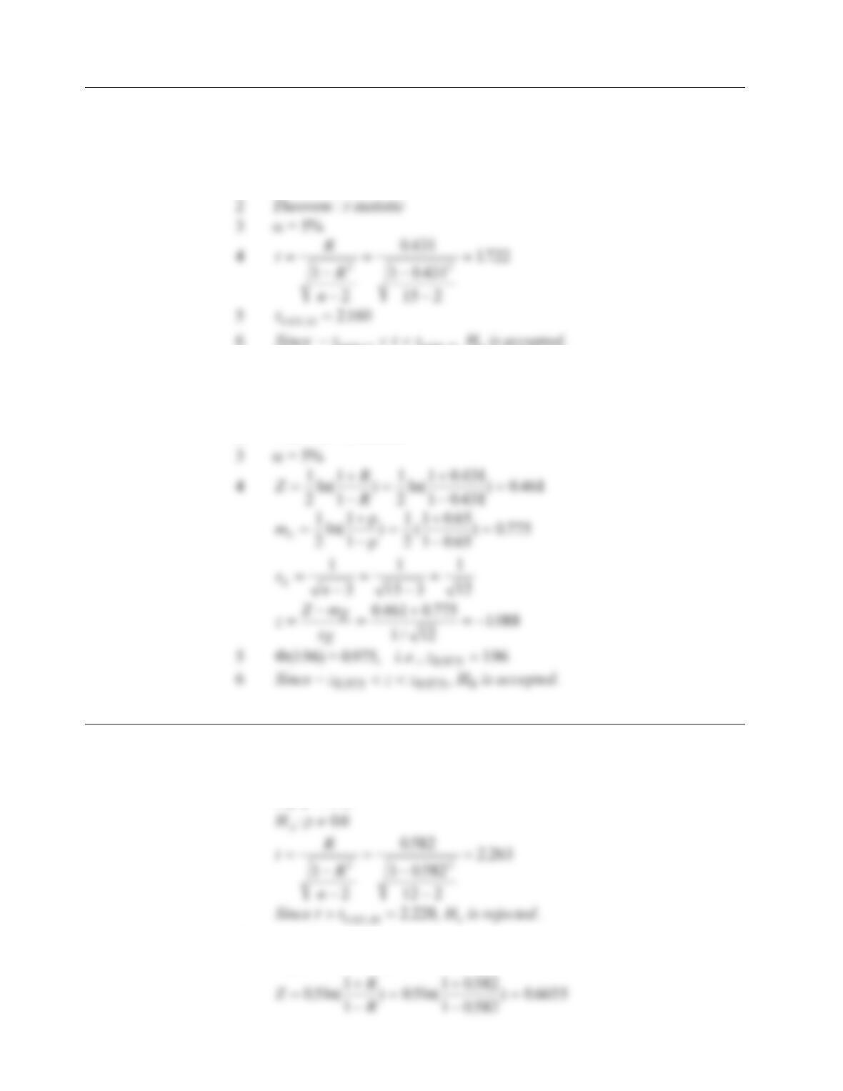
138.10 = sum of products

10.78 = sum of X variation

Problem 12-31.

50.89 = sum of products

4.97 = sum of X variation

12-15

Problem 12-32.

n

R

15 0 431 5%,.,D

(a)

U000 .

1

H000:.U

HA:.Uz00

0 025 13 0 025 13 0., .,, .

(b) U0065 .,

1

H0065:.U

HA:.Uz065

2

Theorem z statistic:

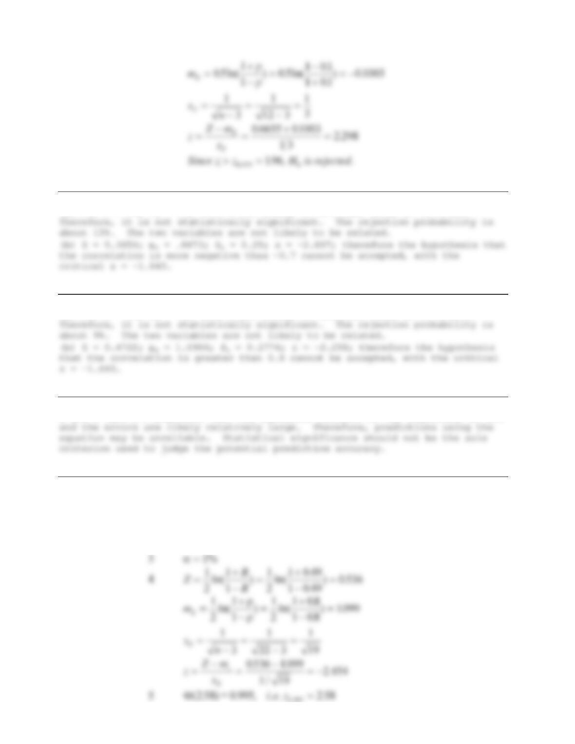
Problem 12-33.

n

R

12 0 582 5%,.,D

(a)

U 00.,

H000:.,U

(b) U 01.,

HH

a001 01:.,:.UU  z

12-16

Problem 12-34.

(a) For n = 19, nu = 17, with a two sided, 5% critical value of +/-0.456.

Problem 12-35.

(a) For n = 16, nu = 14, with a two sided, 5% critical value of +/-0.4973.

Problem 12-36.

A low R (and R2) indicates that the explained variance of the regression is low

Problem 12-37.

U008 22 049 ., , .nR

1

H008:.U

HA:.Uz08

2

Theorem z statistic:

12-17

Problem 12-38.

For degrees of freedom of 8 the critical value is 0.6319. For degrees of

12.3. Introduction to Regression

Problem 12-39.

The slope is 1.327893 with an intercept of zero.

Regression Statistics

Multiple R 0.911879

Problem 12-40.

The slope is 1.004891 with an intercept of zero.

Regression Statistics

Multiple R 0

R Square -0.05237

Problem 12-41.

DATA MATRIX

—————————

Obs. X Y

—- ——— ———

1 .70000 34.00000

12-18

Obs.

no. X( ) YP( ) Y( ) error e / Y

—- ——– ——– ——– ——– ——–

1 .7000 16.4841 34.0000 -17.5159 -.5152

2 1.3000 30.6132 55.0000 -24.3868 -.4434

Problem 12-42.

DATA MATRIX

—————————

Obs. X Y

—- ——— ———

1 1.20000 38.00000

Obs.

no. X( ) YP( ) Y( ) error e / Y

—- ——– ——– ——– ——– ——–

1 1.2000 27.2285 38.0000 -10.7715 -.2835

2 1.6000 36.3047 78.0000 -41.6953 -.5346

3 2.4000 54.4570 55.0000 -.5430 -.0099

12-19

12.4. Principle of Least Squares

Problem 12-43.

a.

x y xy x^2 y^2

1 1 1 1 1

1 2 2 1 4

R = Correlation = 0.97126

Regression Coefficients:

XY nXY

nnn

1



¦¦¦

ii

i

nb

n

b.

x y xy x^2 y^2

1 1 1 1 1

1 2 2 1 4

R = Correlation = 0.40234

Regression Coefficients:

c.