12-20
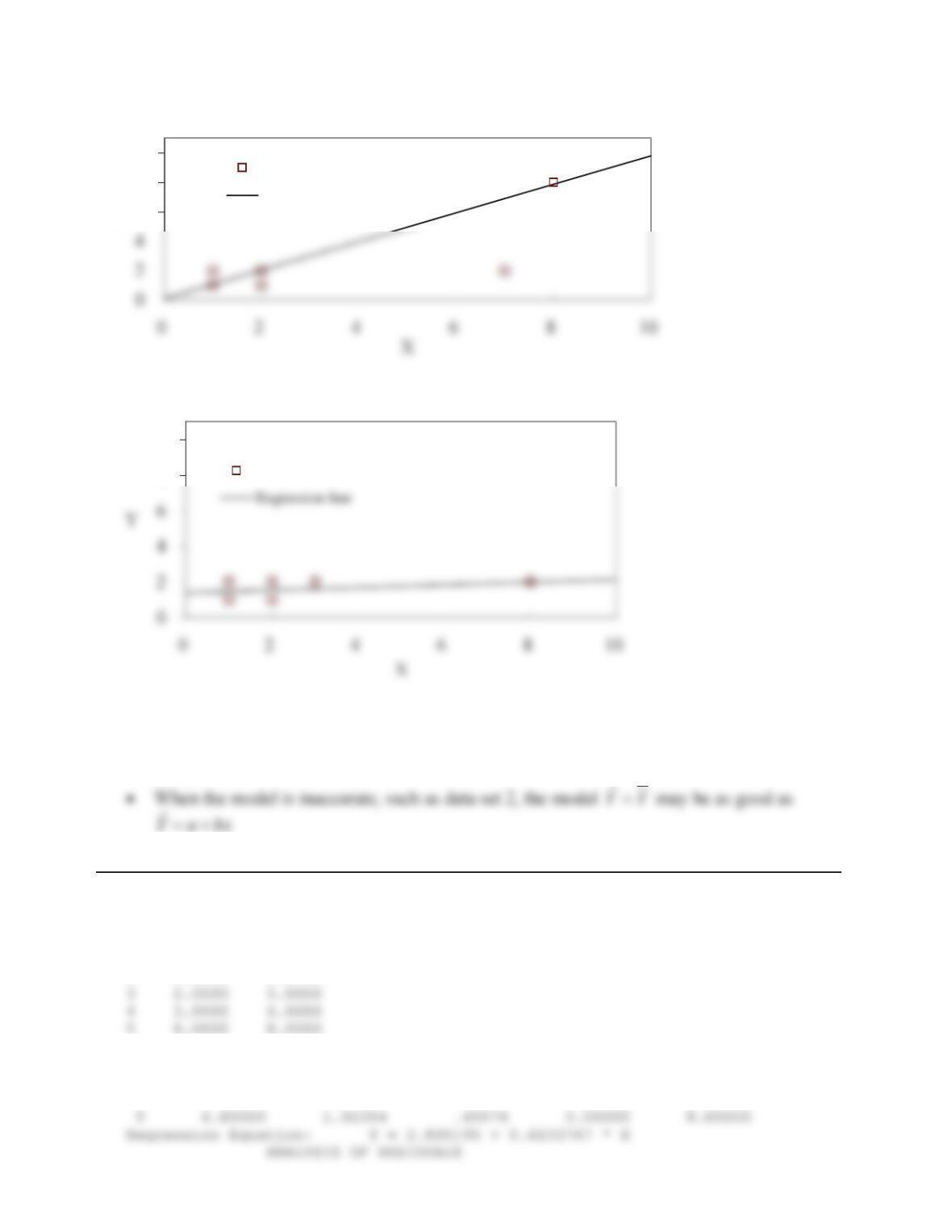
a. Y=0.08046+0.97126X
6
8
10
Y
Observed data
Regression line
b. Y=1.39080+0.07471X
8
10
Observed data
General observations:
xOne point that is an outlier can significantly change the model and goodness of fit
xThe correlation increases when the outlying point is beyond the range of data for both x
and y
Problem 12-44.
Part (a)
DATA MATRIX
———–
1 1.0000 4.0000
2 2.0000 3.0000
Standard Coeff. of Minimum Maximum
Var Mean deviation variation value value
— ———- ———- ———- ———- ———-
X 3.20000 2.77489 .86715 1.00000 8.00000
12-21
——————————————————-
Predicted Observed Error Relative
I YP Y e = YP – Y Error(e/Y)
— ———- ———- ———- ———-
1 3.428571 4.000000 -.571429 -.142857
2 4.051948 3.000000 1.051948 .350649
GOODNESS-OF-FIT CALCULATIONS
—————————-
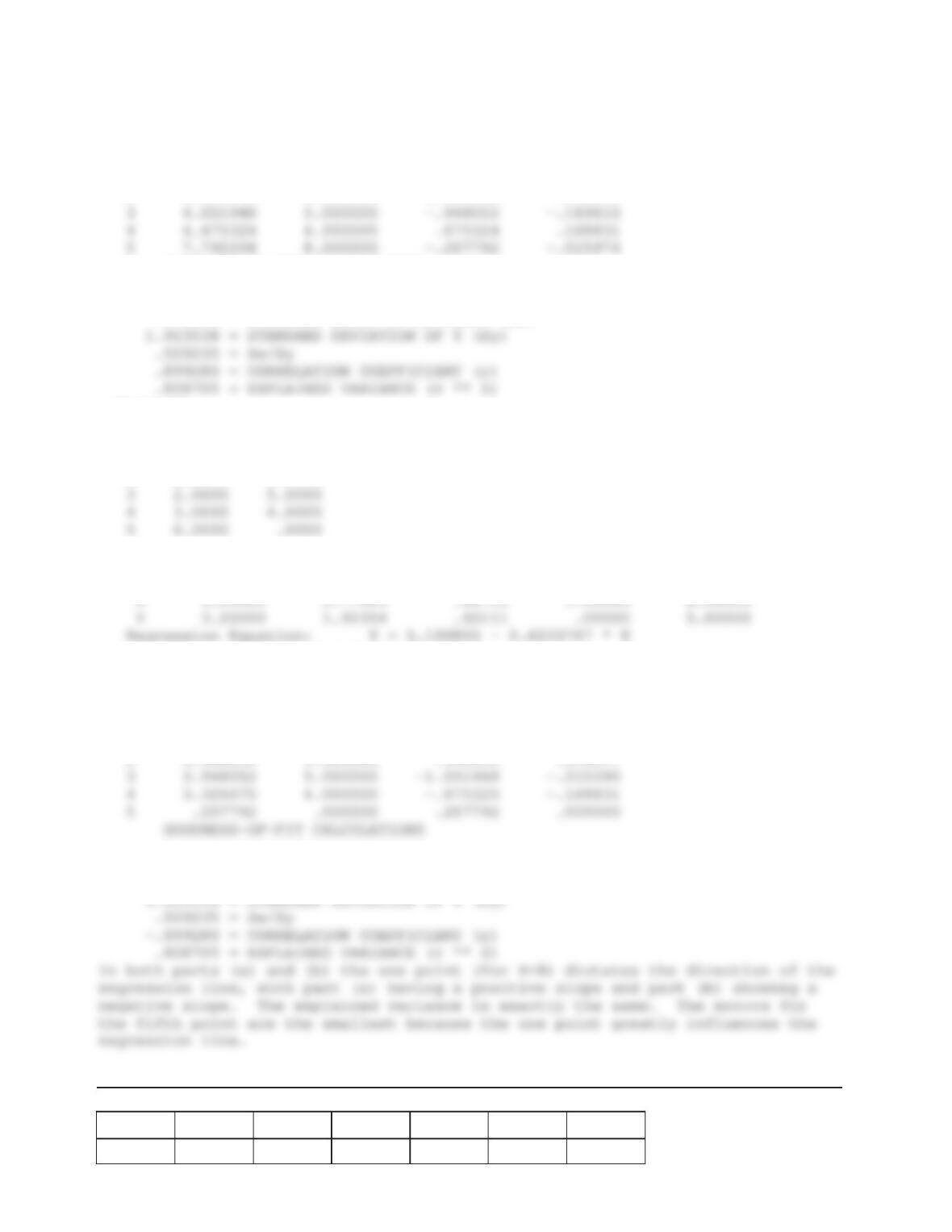
.000000 = BIAS
.971454 = STANDARD ERROR OF ESTIMATE (Se)
Part (b)
DATA MATRIX
———–
1 1.0000 4.0000
2 2.0000 3.0000
Standard Coeff. of Minimum Maximum
Var Mean deviation variation value value
— ———- ———- ———- ———- ———-
ANALYSIS OF RESIDUALS
——————————————————-
Predicted Observed Error Relative
I YP Y e = YP – Y Error(e/Y)
— ———- ———- ———- ———-
1 4.571428 4.000000 .571428 .142857
2 3.948052 3.000000 .948052 .316017
—————————-
.000000 = BIAS
.971454 = STANDARD ERROR OF ESTIMATE (Se)
Problem 12-45.
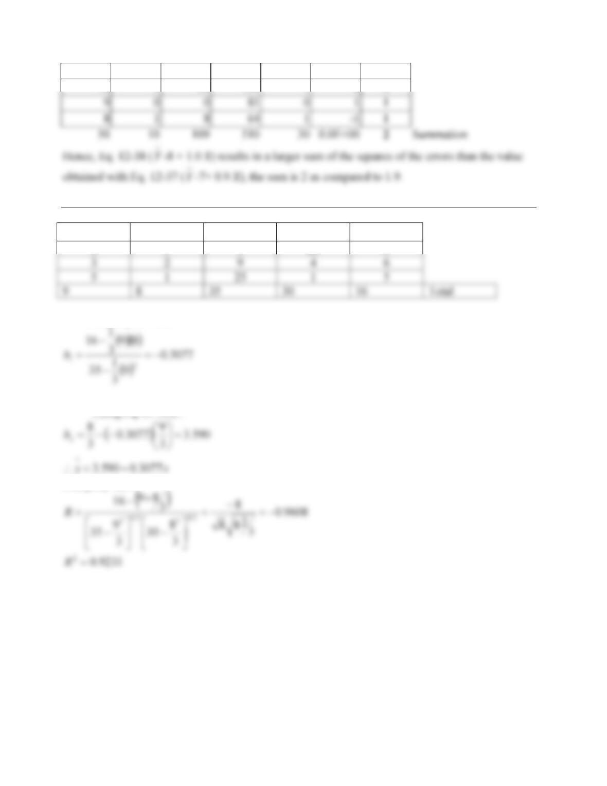
x y xy x^2 y^2 eiei2
12 4 48 144 16 0 0
12-22
11 3 33 121 9 0 0
10 2 20 100 4 0 0
Problem 12-46.
x
y2
x2
y
x
y
1 5 1 25 5
:35a–12Eq.Using
Using Eq. 12-5
12-23
12.5. Reliability of the Regression Equation
Problem 12-47.
a.
b.
x y xy x^2 y^2
3 4 12 9 16
5 8 40 25 64
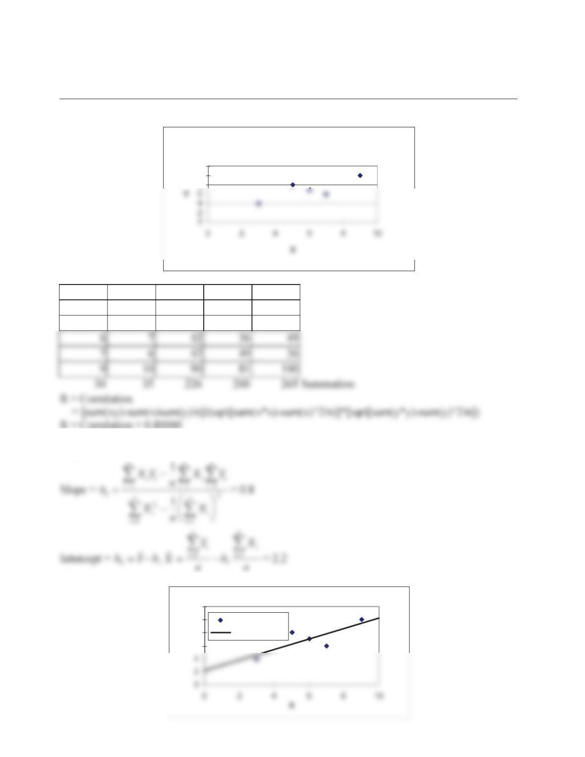
R = Correlation = 0.80000
c.
Regression Coefficients:
d.
8
10
12
6
8
10
12
Y
y
Regression line
12-24
e.
x y y-predicted
3 4 4.6
f.
y y^ y-y^ (y-y^)2
4 4.6 0.6 0.36
8 6.2 -1.8 3.24
g.
Y
Problem 12-48.
DATA MATRIX
———–
1 1.2000 38.0000
2 1.6000 78.0000
Standard Coeff. of Minimum Maximum
Var Mean deviation variation value value
— ———- ———- ———- ———- ———-
12-25
—————————-
.00000 = BIAS
21.221170 = STANDARD ERROR OF ESTIMATE (Se)
25.887120 = STANDARD DEVIATION OF Y (Sy)
34.7 is not too much smaller than the smallest value of Y (38), which suggests
that the intercept is too large. This is often a problem when the correlation
is low.
Problem 12-49.
DATA MATRIX
———–
1 .7000 34.0000
2 1.3000 55.0000
Standard Coeff. of Minimum Maximum
Var Mean deviation variation value value
— ———- ———- ———- ———- ———-
X1 2.12857 .91052 .42776 .70000 3.30000
ANALYSIS OF RESIDUALS
——————————————————-
Predicted Observed Error Relative
I YP Y e = YP – Y Error(e/Y)
— ———- ———- ———- ———-
1 39.957490 34.000000 5.957493 .175220
2 46.095340 55.000000 -8.904655 -.161903
—————————-
.00000 = BIAS
10.575120 = STANDARD ERROR OF ESTIMATE (Se)
13.414630 = STANDARD DEVIATION OF Y (Sy)
12-26
Problem 12-50.
x
y2
x2
y
x
y
ye2
e
3 4 9 16 12 4.6 0.6 0.36
5 8 25 64 40 6.2 -1.8 3.24
6 7 36 49 42 7.0 0 0
The resulting errors (e) are still large. If y was used as the estimate
y, then the Sy of 2.236 would
be a measure of the prediction accuracy. The ye SS / of about 70% indicates that prediction of Y
using the regression equation provides slightly better accuracy.
Problem 12-51.
Se = 1.549 (see Problem 12-28) when Eq. 12-45 is used.
Problem 12-52.
yyy
2
yy
yyy
2
¸
¹
·
¨
©
§
yy
4 -3 9 4.6 2.4 5.76
Problem 12-53.
Using the summations from Problem 12-16,
SS SS SS
ETR
12 616.
MS SS
RR
15 384.
12.6. Reliability of Point Estimates of the Regression Coefficients
Problem 12-54.
8.0)236.2/236.2(8.0/
1
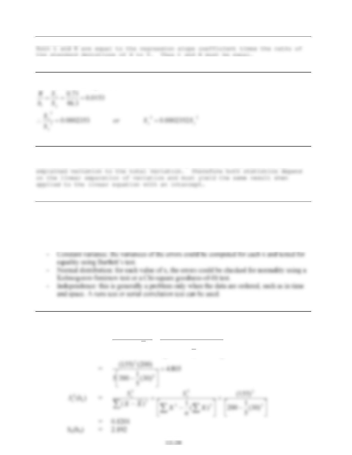
SSbt yx
Problem 12-55.
Problem 12-56.
If t = R, then from Eq. 12-51
Problem 12-57.
The F statistic is the ratio of the mean square between to the mean square of
the error. The correlation coefficient is a function of the ratio of the
Problem 12-58.
The four assumptions are that the residuals, or errors, (1) have a zero mean for any value of y, (2)
have constant variance across values of y, (3) are normally distributed for any value of y, and (4)
are independent of each other. The tests are as follows:
– Zero mean: for any value of x, the errors could be computed and a on-sample t test applied
to assess a zero mean.
Problem 12-59.
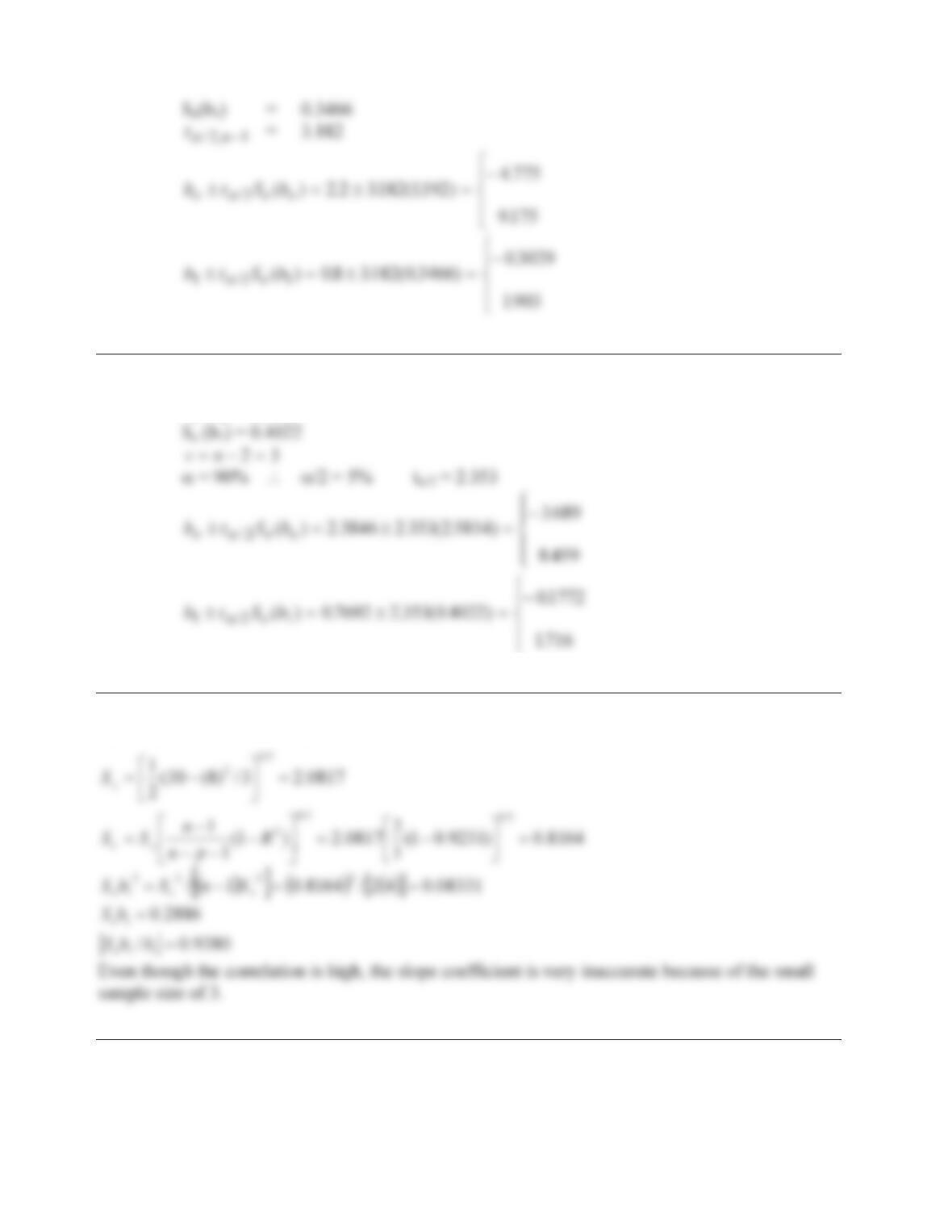
Using the following quantities:
Sb
eo
2()
= SX
nXX
SX
nXnX
ee
22
2
22
22
1
¦
¦¦
¦¦
ª
¬
Ǽ
¼
»
() ()
12-29
Problem 12-60.
b
0 = 2.3846 b1 = 0.7692 Se = 2.0515
S
e (b0) = 2.5814
Problem 12-61.
9231.03077.0
2
1
Rb
Problem 12-62.
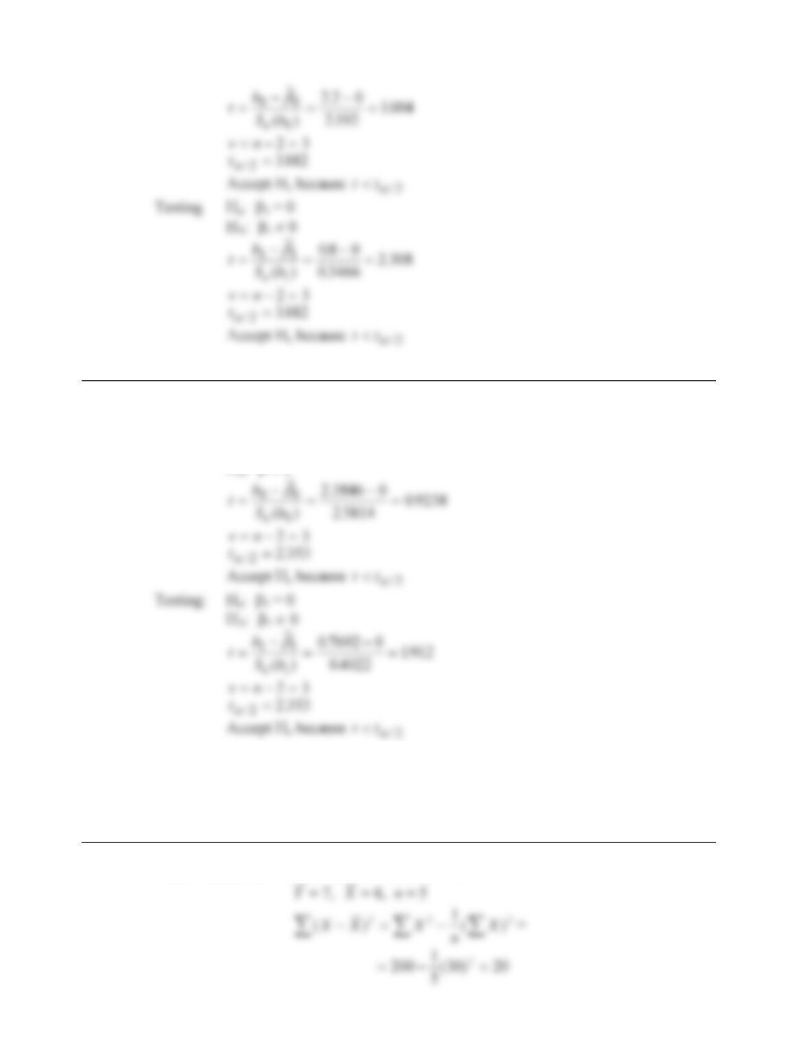
From Problem 12-27: b0 = 2.2, b1 = 0.8
From Problem 12-35: Se (b0) = 2.192, Se (b1) = 0.3466
Testing Ho : Eo = 0
H
A:Eoz 0
12-30
Problem 12-63.
From Problem 12-31: b0 = 2.3846, b1 = 0.7692
From Problem 12-36: Se (b0) = 2.5814, Se (b1) = 0.4022
Testing: Ho:E0 = 0
H
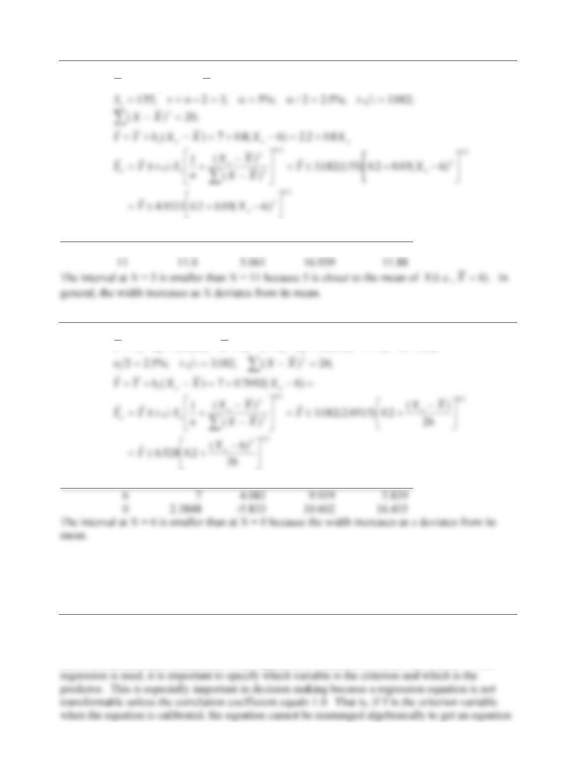
12.7. Confidence Intervals of the Regression Equation
Problem 12-64.
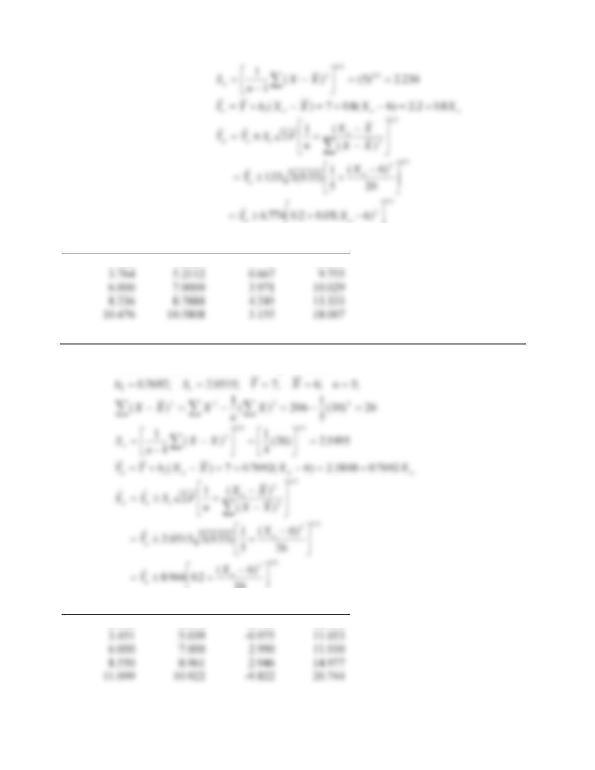
From Problem 12-27: b0 = 2.2, b1 = 0.8, Se = 1.55
12-31
¬
¼
Xa
Ya
Ycl
Ycu
1.528 3.4224 -3.998 10.843
Problem 12-65.
From Problems 12-16, and 12-31 bo 23846.;
¬
¼
26
Xa
Ya
Ycl
Ycu
0.901 3.078 -6.744 12.900
12-32
Problem 12-66.
Yb Xn 70865
1
;.;;;
¬
¼
Xo
Y
YCL
YCU Width
5 6.2 3.983 8.417 4.43
Problem 12-67.
Yb XnS v
7 0 7692 6 5 2 0515 3 5%;
;.;;; .;;D
Xo
Y
YCL
YCU Width
12.8. Correlation Versus Regression
Problem 12-68.
Correlation analysis provides a measure of goodness of fit; whereas regression analysis is a mean
of calibrating the unknown coefficients of a prediction equation. Correlation has its usefulness in
model formulation and verification, while regression is a method for model calibration. When
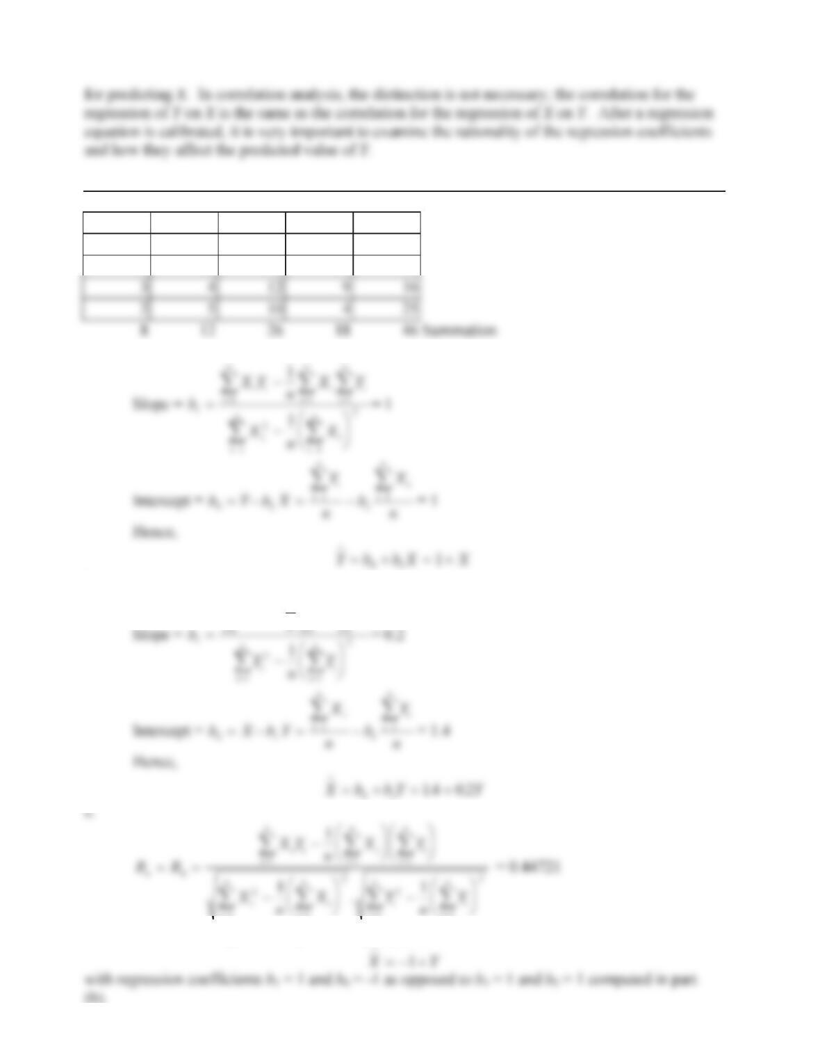
12-33
Problem 12-69.
x y xy x^2 y^2
2 1 2 4 1
1 2 2 1 4
a.
b.
XY nXY
nnn
1
¦¦¦
ii
i
i
i=1
i=1
i=1
i=1
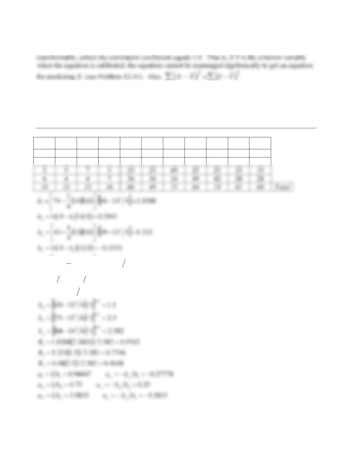
d. The transformed regression equation of part (a) is
(b).
12-34
e. When using regression, it is necessary to specify which variable is the criterion and which is the
predictor. The distinction is necessary with regression because a regression equation is not
12.9. Applications of Bivariate Regression Analysis
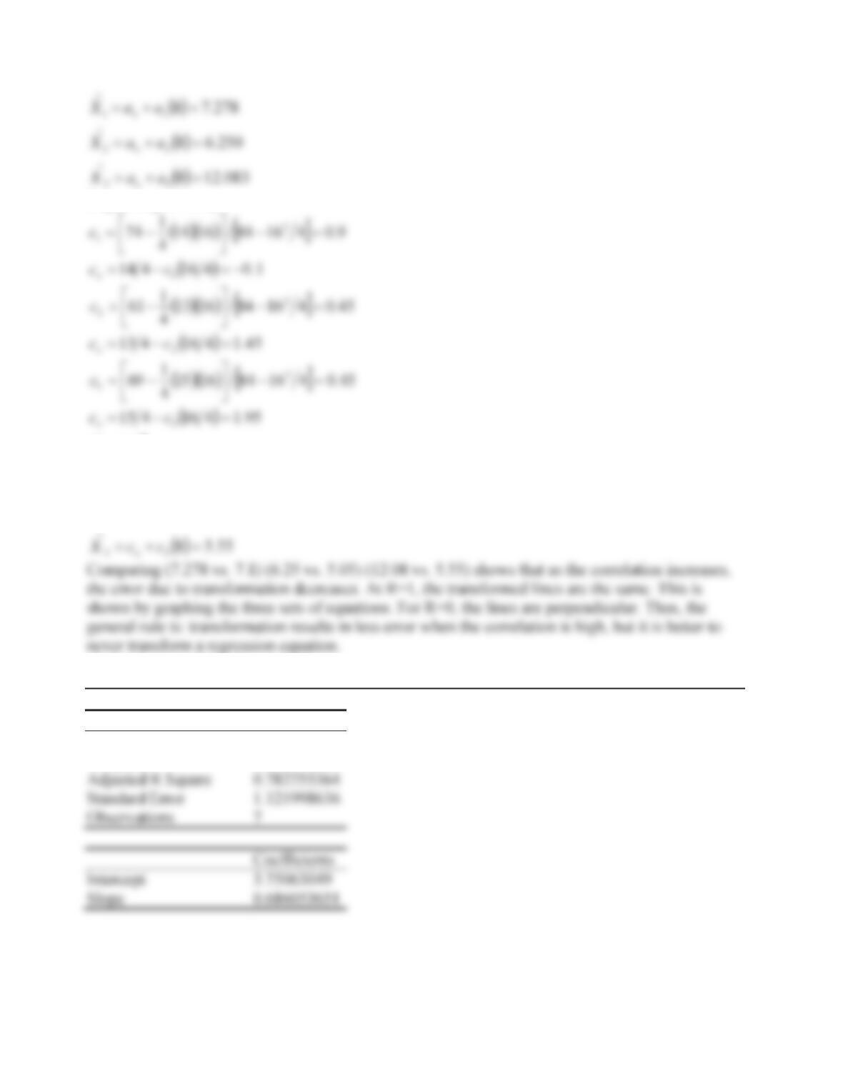
Problem 12-70.
1
x2
x3
xy2
1
x2
2
x2
3
x2
yyx1yx2yx3
1 2 3 1 1 4 9 1 1 2 3
2 2 1 3 4 4 1 9 6 6 3
>@
2.2415416
48.041575/1615
4
1
69
3
2
3
»
¼
º
«
¬
ª
bb
b
o
>@
3805.23/41466
5.0
2
1
S
12-35
Regressing x’s on y
05.58
1.78
8
22
11
ccX
ccX
yat
o
o
Problem 12-71.
Regression Statistics
Multiple R 0.904965637
R Square 0.818962804
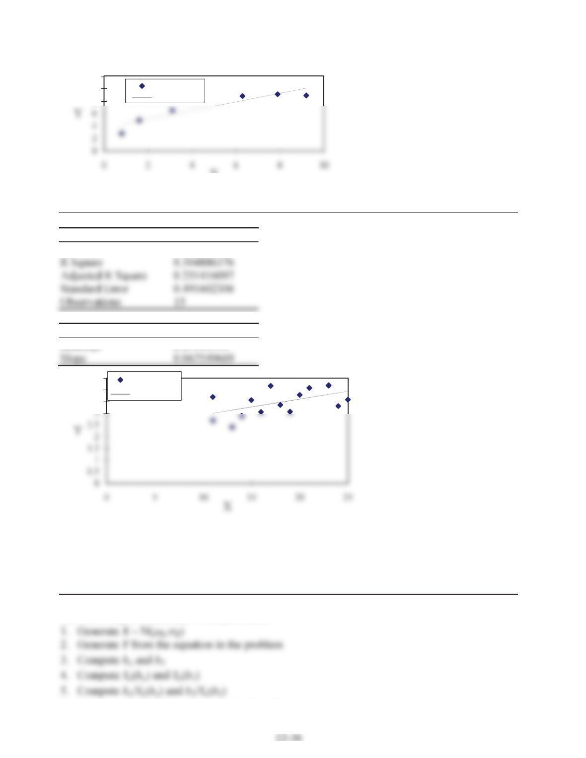
8
10
12
X
Y
Predicted Y
Problem 12-72.
Regression Statistics
Multiple R 0.552165171
Coefficients
Intercept 2.25010596
3.5
4
4.5
Y
Predicted Y
12.10. Simulation and Prediction Models
Problem 12-73.
The following is a summary of the procedure:
Both histograms should have a central value of t
D
/2,n-2.

12-37
Problem 12-74.
The standard error (Se) is 0.02495
The following results can be obtained:
D (%) Critical value
3.032