14-1
Solutions for Chapter 14 – Models for Non-ideal
Reactors
P14-1 Individualized solution
P14-2 (a)
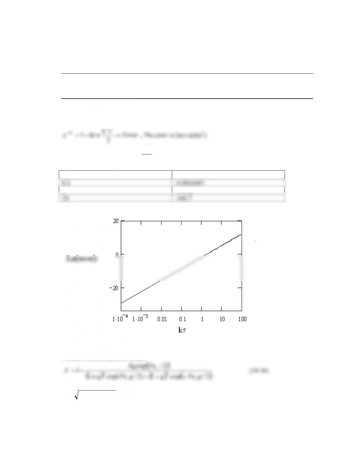
Approximated formula for Segregation Model (1st reaction)
Error
tk
kte kt ++!=
!
2
1
22
. The error is then o((kt)3).
Approximating the
!3
3
kt
Error !=
!
k
Error
0.1
-0.0001667
1
-0.1667
10
-166.7
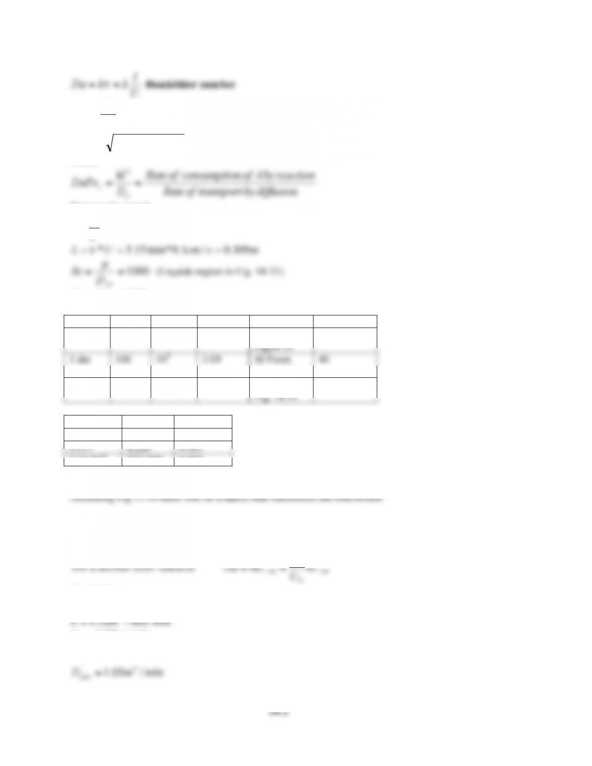
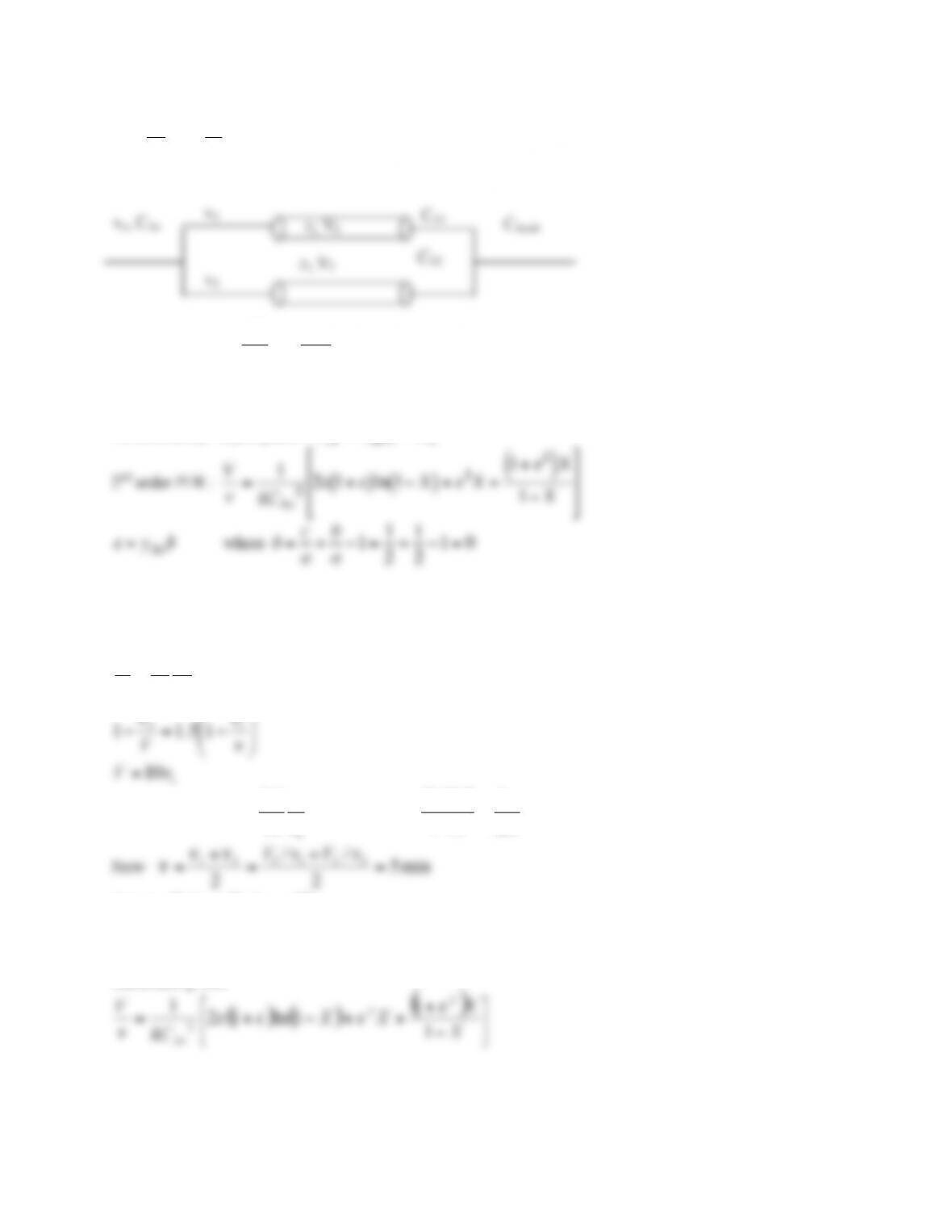
P14-2 (b)
Parameters Dispersion Model
Closed-Closed dispersion model
( )
( ) ( ) ( )
2/exp1)2/exp(1
2/exp4
122 qPeqqPeq
Peq
X
rr
r
!!!+
!=
(14-26)
Where
r
PeDaq /41 +=
U
l
kkDa ==
!
Damköhler number
a
rD
Ul
Pe =
Peclet number
rr DaPePeqPe 4
2
2+=
Where
diffusionbytransportofRate
reactionbyAofnconsumptioofRate
D
kl
DaPe
a
r==
2
Numerical example
min.155=== const
U
L
!
mscmUL 309.0/1.0min*15.5* ===
!
1000==
AB
D
Sc
µ
(Liquids region in Fig. 14.11)
2881.==
!
kDa
dt
Re
ReSc
L/dt
D/(U*dt)
D (cm2/s)
1 cm
10
104
30.9
0.18 From
Fig14.10
0.018
1 dm
100
105
3.09
40 From
Fig. 14.11
40
Per
Q
X
0.077
8.226
0.567
1.03·10-4
223.609
0.563
According Fig.14.10 there will be a radius that maximizes the conversion.
P14-2 (c)
For a second order reaction
0
0
0AA kC
U
L
kCDa ==
!
mR 05.0=
Damköhler number/ Da
Conversion
Parameter
0.1603
0.138
8*U0
0.3205
0.239
4*U0
0.641
0.377
2*U0
1.282
0.523
U0
2.564
0.644
U0/2
5.129
0.732
U0/4
10.258
0.795
U0/8
(2) Vary the Peclet and Damköhler numbers for a second–order reaction in laminar flow
(Example 14–3(c))
For a second order reaction
0
0
0AA kC
U
L
kCDa ==
!
;
AB
DLUPe /
0
=
mR 05.0=
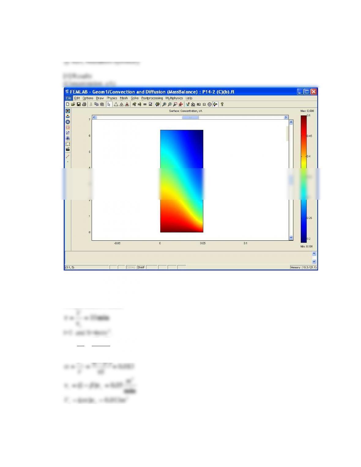
Below is a FEMLAB anaylsis of the problem.
(1) Vary the Damköhler number for a second–order reaction (Example 14–3(b))
For a second order reaction
0
0
0AA kC
U
L
kCDa ==
!
mR 05.0=
14-5
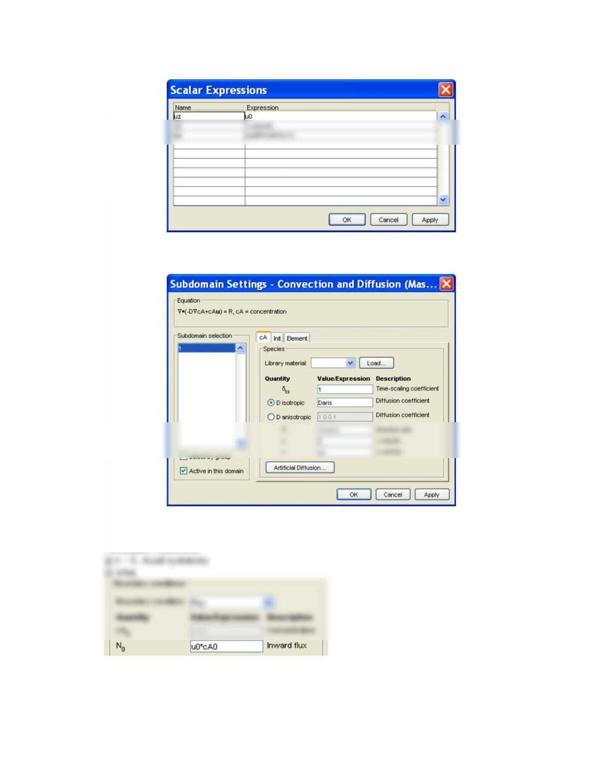
– Scalar expressions
[3] Subdomain Settings
– Physics
(Mass Balance)
– Initial Values
(Mass balance) cA(t0) = cA0
– Boundary Conditions
@ r = 0, Axial symmetry
@ inlet,
@ outlet, Convective flux
@ wall, Insulation/Symmetry
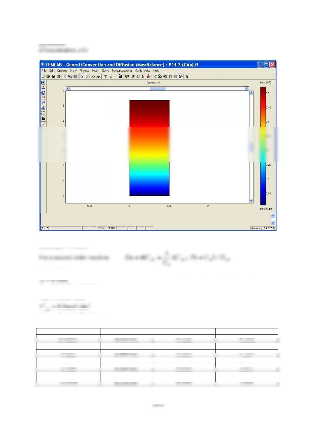
[4] Results
(Concentration, cA)
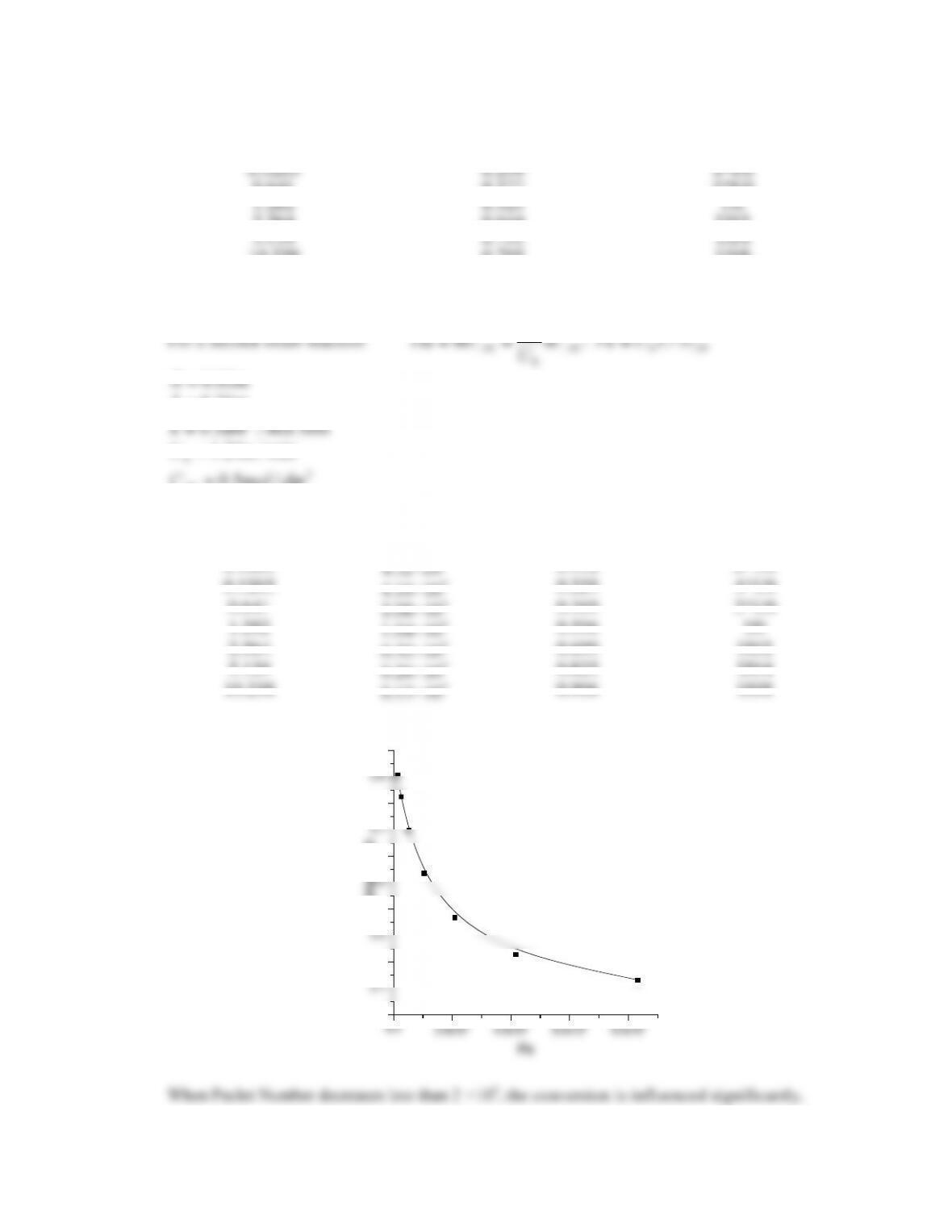
(2) Vary the Peclet and Damköhler numbers for a second–order reaction in laminar flow
(Example 14–3(c))
For a second order reaction
0
0
0AA kC
U
L
kCDa ==
!
;
AB
DLUPe /
0
=
min./5.0 3moldmk =
min/24.1
0mU =
3
0/5.0 dmmolC A=
min/106.7 25 mDAB
!
“=
Da
Pe
Conversion
Parameter
0.1603
8.32×10⁵
0.132
8*U0
0.3205
4.16×10⁵
0.229
4*U0
0.641
2.08×10⁵
0.369
2*U0
2.564
0.52×10⁵
0.699
U0/2
10.258
0.13×10⁵
0.906
U0/8
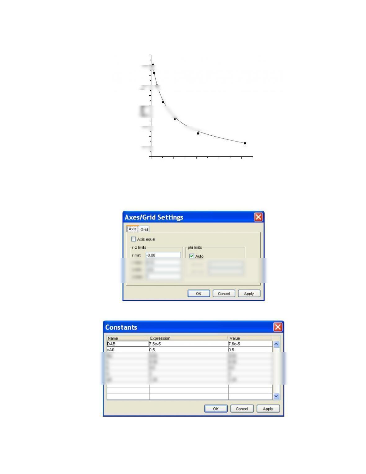
14-7
0.0 2.0x1054.0x1056.0x1058.0x105
0.0
0.1
0.2
0.3
0.4
0.5
0.6
0.7
0.8
0.9
1.0
Conversion
Pe
When Peclet Number decreases less than 2 ×10⁵, the conversion is influenced significantly.
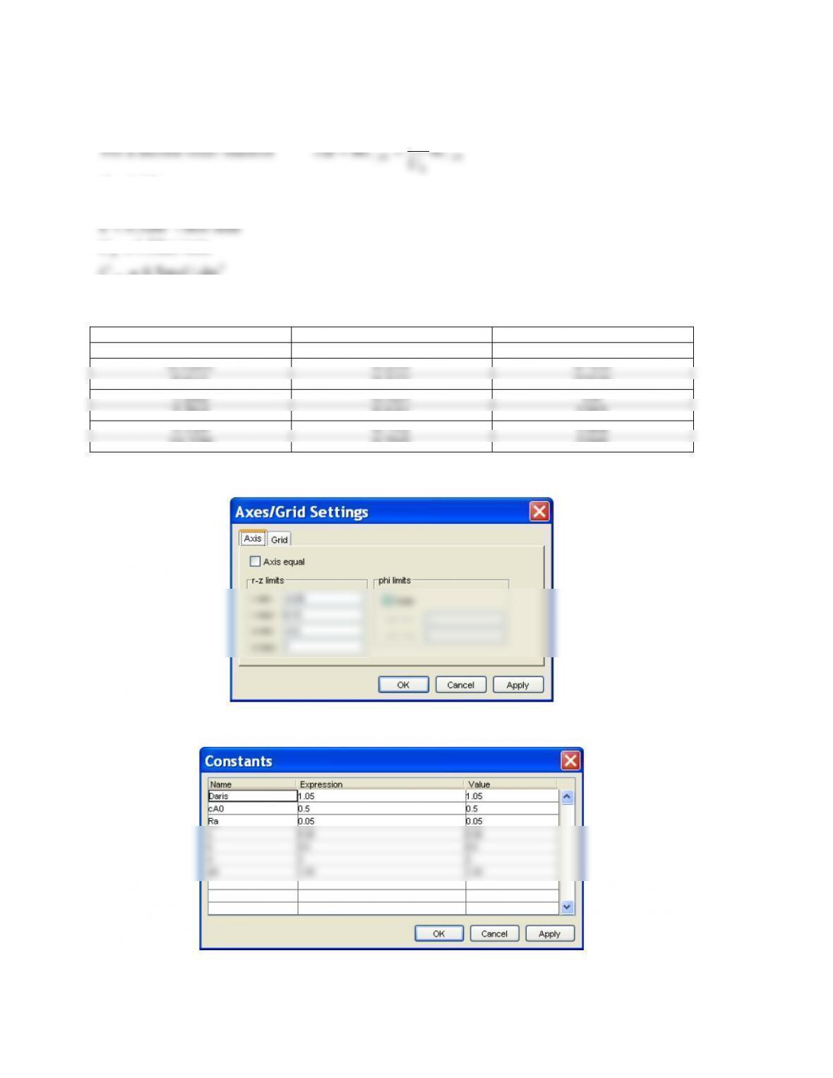
– Femlab Screen Shots
[1] Domain
[2] Constants and scalar expressions
– Constants
14-8
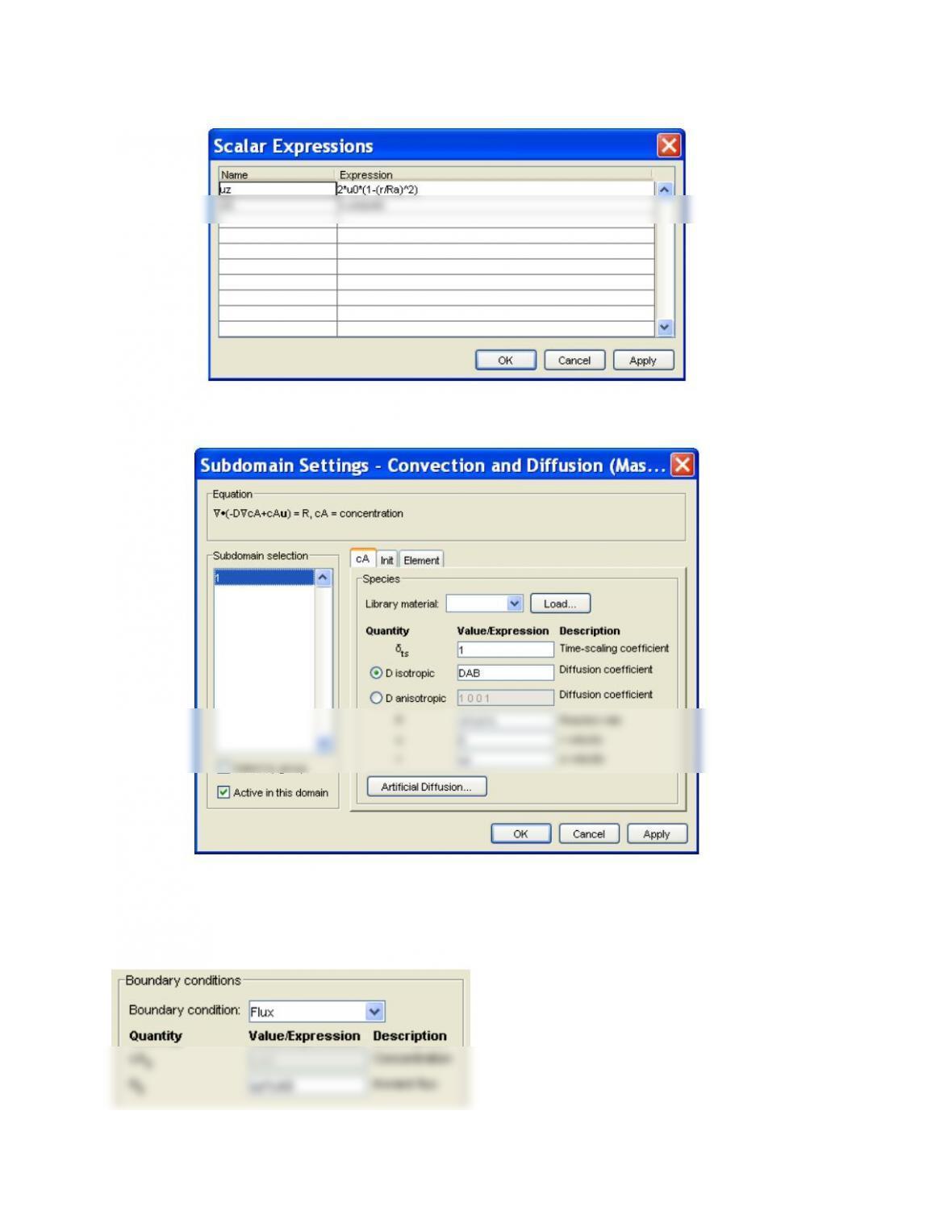
– Scalar expressions
[3] Subdomain Settings
– Physics
(Mass Balance)
– Initial Values
(Mass balance) cA(t0) = cA0
– Boundary Conditions
@ r = 0, Axial symmetry
@ inlet,
14-9
@ outlet, Convective flux
@ wall, Insulation/Symmetry
[4] Results
P14-2 (d)
Two parameters model
min10==
o
v
V
!
I=2 and S=4min-1.
50
1.
)( =
!
== I
I
v
v
o
b
“
( ) 0130
1.=
!
== SV
Vs
“
#
$
min
.)(
3
0501 m
vv os =!=
“
3
0130 mvV os .)( ==
!”
14-10
min.250==
s
s
sv
V
!
3
7791
2
141
m
kmol
k
kC
C
Aos
As .=
!+
=
“
“
Bypass
(I=1.25 and S=0.115 min-1)
Bypass
(I=2.0 and S=4 min-1)
X=0.66
X=0.51
X=0.111
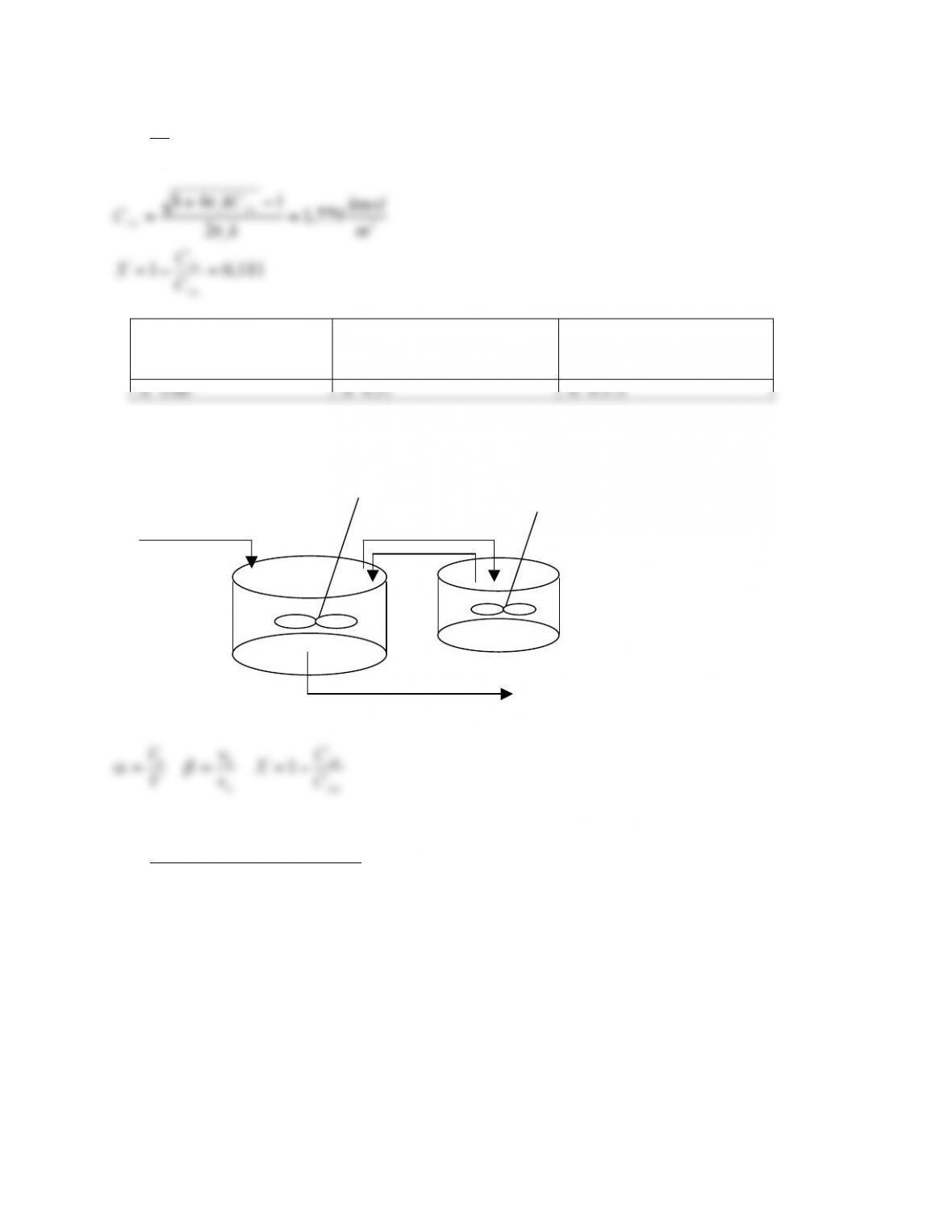
P14-2 (e)
Ao
A
oC
C
X
v
v
V
V111 1!===
“#
( ) ( )
[ ]
( ) tk
tktk
X
!“
“!“!“
+#
##++
=1
12
See Polymath program P14-2-e.pol
v1
V1
v1
V2
CA0 v0
CA1 v0
14-11
POLYMATH Results
Calculated values of the DEQ variables
Variable initial value minimal value maximal value final value
t 0 0 200 200
CT1 2000 31.814045 2000 31.814045
CT2 921 164.15831 1048.4628 164.15831
beta 0.15 0.15 0.15 0.15
alpha 0.75 0.75 0.75 0.75
CTe2 921 13 921 13
t1 -80 -80 120 120
CTe 2000 13 2000 13
Differential equations as entered by the user
[1] d(CT1)/d(t) = (beta*CT2-(1+beta)*CT1)/alpha/tau
[2] d(CT2)/d(t) = (beta*CT1-beta*CT2)/(1-alpha)/tau
Explicit equations as entered by the user
[1] beta = 0.15
[2] alpha = 0.75
[3] tau = 40
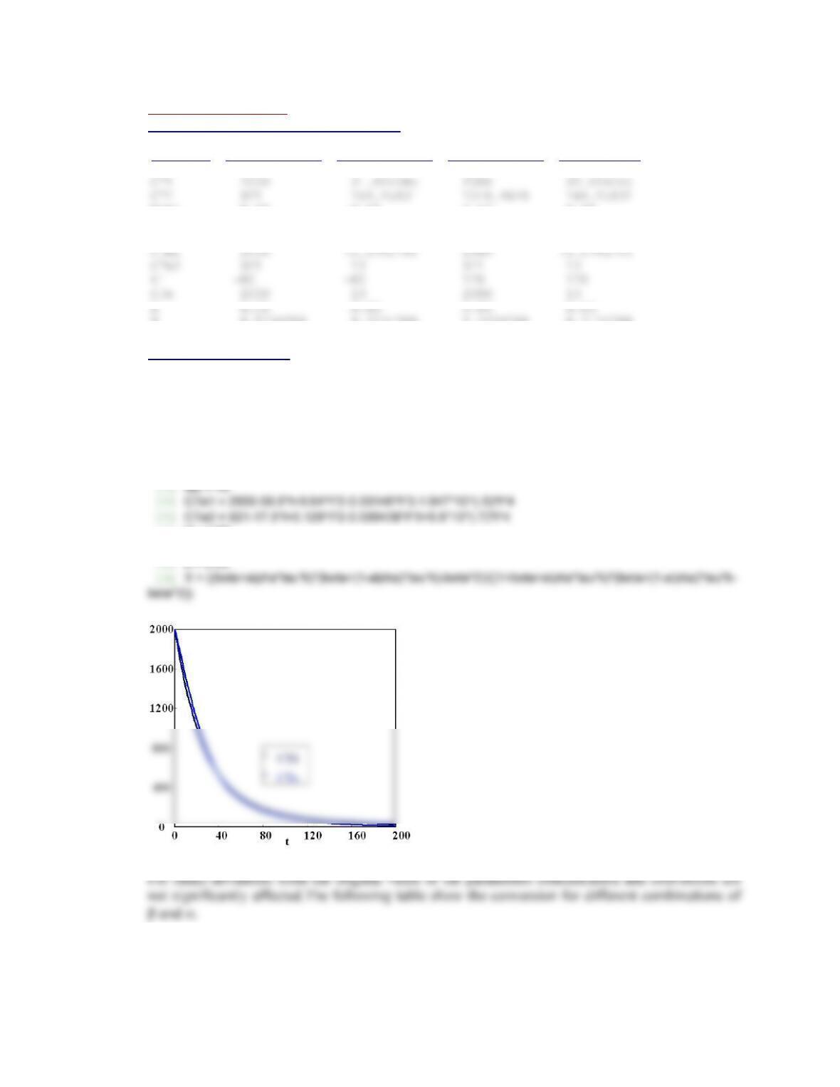
[4] CTe1 = 2000-59.6*t+0.64*t^2-0.00146*t^3-1.047*10^(-5)*t^4
[5] CTe2 = 921-17.3*t+0.129*t^2-0.000438*t^3+5.6*10^(-7)*t^4
[6] t1 = t-80
[9] X = ((beta+alpha*tau*k)*(beta+(1-alpha)*tau*k)-beta^2)/((1+beta+alpha*tau*k)*(beta+(1-alpha)*tau*k-
beta^2))
Comparison experimental and predicted (β=0.15 α=0.75) concetration.
For small deviations from the original value of the parameters concentration and conversion are
not significantly affected.The following table show the conversion for different combinations of
β and α.
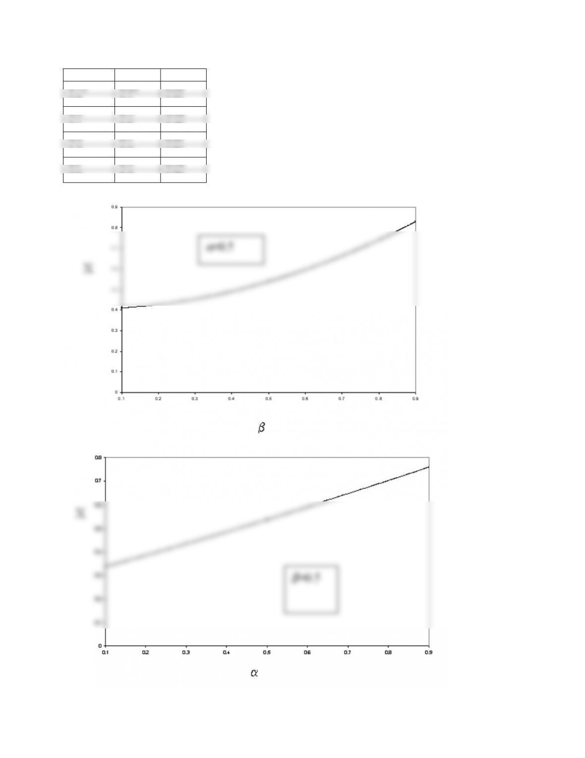
14-12
α
β
X
0.75
0.15
0.51
0.8
0.1
0.51
0.5
0.5
0.54
0.5
0.1
0.41
0.1
0.5
0.34
14-13
Given the interchange flowrate, the conversion is increased with the increasing of the volume of
the highly agitated reactor. Given the volume of the highly agitated reactor, the conversion is
increased with the increasing of the interchange.
The correlations between Re and Da show what flow conditions (characterised by Re) give the
greatest or smallest Da and hence dispersion.
To minimise dispersion a Re number of ~10-20 gives the lowest value for Da. Because
Re =
“
ud
µ
,
May be a good approximation if CA does not change very much with time, i.e. A is in excess, in
which case CAo should not be divided by anything.
Linearizing the non 1st order reactions may give significantly inaccurate results using Equation
The curves in Fig.14.3 represent the residence time distributions for the Tanks in Series model as
function of the number of reactors.
Given a CSTR of volume 1 (V=V1), we divide the CSTR in two CSTRs (V2=1/2). The mean
residence time is unchanged (V/F) but the molecules going out of the second reactor will be
delayed by the time (distribution) that occur to pass the first reactor (n=2, shift of the maximum).
In the limit of infinite division (Vn=0), so in the single CSTRs the residence time goes to zero for
all the molecules (zero variance), but their summation is the mean residence time (n=∞, PFR
the real reactor for less than time t shows a step up from zero when flow leaves from the “faster”
reactor. This fraction is the fraction of flow in the “slower” reactor. When the flow leaves the
“slower” reactor this fraction becomes one.
The model in Fig. 14.1 is PFR and CSTR in parallel. The exit age distribution for the CSTR is a
Conversion
5.0
1==
!
“
#
5.1
1
1
2=
!
!
=
“
#
$
14-14
V
V1
=
!
v
v1
=
!
r2, V2
Rate law:
2
AA kCr =!
Stoichiometry: liquid phase
CA=CAo 1“X
( )
2nd order PFR :
V
v=1
kCAo
22
“
1+
“
( )
ln 1#X
( )
+
“
2X+
1+
“
2
( )
X
1#X
$
%
&
&
‘
(
)
)
Determining
!
and
!
:
5.0
1
1== v
v
V
Vo
!
“
→
11 5.2 vV =
!
“
#
$
%
&‘=‘v
v
V
V11 15.11
1
10vV =
Gives
25.0
10
5.2
1
== v
vi
!
and
50
52
5
5
52
1.
./
./ ===
!
“
V
V
Now
min5
2
//
2
221121 =
+
=
+
=vVvV
!!
!
Hence
10// 2211 =+ vVvV
11 5.2 vV =
22 5.7 vV =
Gives
min5.2
1=
!
min5.7
2=
!
Substituting into
( ) ( ) ( ) !
“
#
$
%
&
‘
+
++‘+= X
X
XX
kC
v
V
Ao 1
1
1ln12
12
2
2
(
(((
CAexit
v1
vo, CAo
CA1
r1, V1
Reactor 1:
!
“
#
$
%
&
‘
=
1
1
21210
1
52
X
X
*.
.
!
“
#
$
%
&
‘
=
1
1
1
1
X
X
→
5.0
1=X
( ) ( ) 3
11 /15.0121 dmmolXCC AoA =!=!=
Reactor 2:
!
“
#
$
%
&
‘
=
2
2
21
2*1.0
1
5.7
X
X
!
“
#
$
%
&
‘
=
2
2
21
2*1.0
1
3
X
X
→
75.0
2=X
( ) ( ) 3
22 /5.075.0121 dmmolXCC AoA =!=!=
3
21 /75.0
2
5.01
2
dmmol
CC
CAA
Aexit =
+
=
+
=
3
/625.0
2
75.02 dmmol
C
CC
X
Ao
AAo =
!
=
!
=
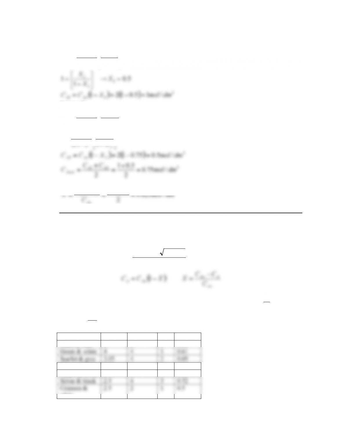
P14-3 (a)
Money for buying reactors
Using the tank in series model:
Second order reaction
Da
DaDa
X
2
1412 +!+
=
where Da=kτCao
( )
XCC AoA !=1
Ao
AAo
C
CC
X!
=
Assume that
t
!!
=
and that in reactors medelled as more than one tank, that
n
t
!
!
=
. Number of
tanks
2
2
!
“
=n
rounded to the nearest integer.
Reactor
Σ(min)
τ(min)
n
X
Maze & blue
2
2
1
0.50
Green & white
4
4
1
0.61
Scarlet & grey
3.05
4
2
0.69
Orange & blue
2.31
4
3
0.72
Crimson &
white
2.5
2
1
0.5
Where
Scarlet & grey: X1 = 0.5, CA1=0.5 → X2 = 0.38, CA2=0.31→ X = 0.69
Orange & blue : X1 = 0.43, CA1=0.57 → X2 = 0.34, CA2=0.38→ X3 = 0.27,
X1 = 0.5, CA1=0.5 → X2 = 0.17, CA2=0.41→ X=0.59
The orange & blue or silver & black reactors which both approximate to 3 tanks in series give the
Try:
Green & white and Maze & blue: X1 = 0.61, CA1=0.39 → X2 = 0.34, CA2=0.26→ X = 0.74
Scarlet & grey and Maze & blue: X1 = 0.69, CA1=0.31 → X2 = 0.42, CA2=0.18→ X = 0.82
& blue reactor.
P14-3 (c)
Ann Arbor, MI
East Lansing, MI
Columbus, OH
Madison, WI
P14-4
Packed bed reactor with dispersion
1st order, k1=0.0167/s, ε=0.5, dp=0.1 cm,
scm /01.0 2
==
!
µ
“
L=10 cm, U= 1 cm/s
10Re ==
µ
!
p
Ud
and
AB
D
Sc
!
=
no data concerning
AB
D
From packed bed correlation for
a
D
, and liquid phase region of graph,
Gives
approx
Ud
D
p
a2=
!
→
scm
Ud
Dp
a/4.0
5.0
1.0*1*2
22
===
!
25
10*1 ===
UL
Pe
14-17
r
Pe
Da
q4
1+=
Da=τκ and
s
U
L10
1
10 ===
!
→ Da=0.167 and q=1.013
15.0=X
Conversion X=15%.
Number of tanks in series
Assuming the Peclet-Bodenstein relation:
1
2+= Bo
n
Where
a
D
UL
Bo =
To estimate
Bo
,
1000
01.0
2*5
Re === v
udt
and
2
005.0
01.0 ===
AB
D
Sc
!
From gas phase dispersion correlation chart,
8=
a
D
5
80
200*2 ==Bo
5.31
2
5=+=n
Reactor 1:
Mol balance:
Ao
A
F
Vr
X!=
Rate law:
2
AA kCr =!
Stoichiometry:
( )
1
1XCC AoA !=
δ=0 and ε=0 hence no volume
change
( ) ( )2
1
2
1
2
11
039.0
01.0*25
1X
vC
XkC
Ao
Ao !=
!
( ) 674.01366.6 2
11 !“=XX
( ) 3
11 /00326.01 dmmolXCC AoA =!=
14-18
Reactor 2:
( ) 507.0
1
2
2
21
2=!
“
=X
v
XkC
XA
( ) 3
212 /001607.0)507.01(00326.01 dmmolXCC AA =!=!=
Reactor 3:
( ) 387.0
1
3
2
32
3=!
“
=X
v
XkC
XA
( ) 3
323 /000985.0)387.01(001607.01 dmmolXCC AA =!=!=
Reactor 4:
( ) 305.0
1
4
2
43
4=!
“
=X
v
XkC
XA
( ) 3
434 /000685.0)305.01(000985.01 dmmolXCC AA =!=!=
Bounds on conversion:
3 tanks
9015.0
3=
!
=
Ao
AAo
C
CC
X
4 tanks
9315.0
3=
!
=
Ao
AAo
C
CC
X
Change of the fluid velocity
Let U=0.1cm/s
Re=50 and Sc=2
From gas phase dispersion correlation chart,
5.0=
t
a
ud
D
Gives
scmudD ta /25.05*1.0*5.05.0 2
===
80
25.0
200*1.0 ===
a
D
UL
Bo
411
2=+= Bo
n
The conversion is close to the one PFR 2nd order reaction:
k=25dm3/(mol·s)
τ=l/U=2/0.001=2000s
Da=kτCAo=500
998.0
=Da
Da
X
Let U=100cm/s
Re=50000 and Sc=2
From gas phase dispersion correlation chart,
21.0=
a
D
gives
scmudD ta /25.05*100*21.021.0 2
===
5.190
105
200*100 ===
a
D
UL
Bo
961
2
5.190
1
2=+=+= Bo
n
The conversion is close to the one PFR 2nd order reaction:
k=25dm3/(mol·s)
τ=l/U=2/1=2s
Da=kτCAo=0.5
1=
+
P14-5 (d)
Change of the superficial velocity
80
01.0
4*2.0
Re === v
udt
From packed bed dispersion correlation chart,
55.0=
p
a
ud
D
!
1.1
4.0
2.0*4*55.0
55.0
===
!
p
a
ud
D
727
1.1
200*4 ===
a
D
UL
Bo
5.3641
2
727
1
2=+=+= Bo
n
The conversion is close to the one PFR 2nd order reaction:
check
k=25dm3/(mol·s)
τ=l/U=2/1=2s
Da=kτCAo=0.5
14-20
P14-6 (a)
Peclet numbers
From Example 13.2 σ2=6.19min2 and tm=5.15min
Closed:
( ) 414.71
22
22
2
=!““=“
r
Pe
r
r
Pee
Pe
Pe
tm
r
#
Open:
68.11
82
22
2
=!+= r
r
r
Pe
Pe
Pe
tm
“
P14-6 (b)
Space–time and dead volume
40.4
21 =
+
=
r
Pe
tm
!
3
8.263* dmvV os ==
!
3
2.156 dmVVV sD =!=
%2.37
420
2.156
%==deadvolume
P14-6 (c)
Conversions for 1st order isomerization
Dispersion model
Da=kτ=0.927
1221
4
1=+=
r
Pe
Da
q
( )
( ) ( ) ( ) ( ) 570.0
2/exp12/exp1
2/exp4
122 =
!!!+
!=
qPeqqPeq
Peq
X
rr
r
Tanks-in-series
35.4
2
2
==
!
“
n
( ) 5680
1
1
1.=
+
!=n
iK
X
“
P14-6 (d)
Conversions PFR and CSTR
PFR:
!
k
eX “
“=1
X=0.604
CSTR:
k
X
!
+
“=1
1
1
X=0.481
XDisp
XT-I-S
XPFR
XCSTR
0.570
0.568
0.604
0.481