10-1
Solutions for Chapter 10 – Catalysis and Catalytic
Reactors
P10-1 Individualized solution
P10-2 (a) Example 10-1
(1) Pentane isomerization
Pt
nP iP!!“
Assume that Pt is the catalyst used.
Maximum f = 5 molecules/site/sec
Maximum rate:
1 %
100
P
Pt
Pt
r fD MW
! “
#=$ %
& ‘
( ) 4
1 1
5 0.5 1.28*10
195 100
P
mol
rs gcat
!
” #
!= =
$ %
& ‘
Minimum:
( )
3 7
1 1
3*10 0.5 7.69 *10
195 100
P
mol
rs gcat
! !
” #
!= =
$ %
& ‘
(2)
2 2 3
1
2
SO O SO+!
No turnover frequency is given so this rate law cannot be determined by this method
Assume Cobalt is the catalyst.
2
1 %
100
H
Co
Co
r fD MW
! “
#=$ %
& ‘
Maximum:
f = 100 molecules/site/sec
( )
2
1 1
100 0.5 0.00849
58.9 100
H
mol
rs gcat
! “
#= =
$ %
& ‘
Minumum:
f = 0.01
( )
2
7
1 1
0.01 0.5 8.49 *10
58.9 100
H
mol
rs gcat
!
” #
!= =
$ %
& ‘
10-2
P10-2 (b) Example 10-2
(1)
1
1
V
C
C K P K P
=+ +
1.39
B
K=
1.038
T
K=
0 0 0.3* 40 12
T T Total
P y P= = =
For 60% conversion
( )
01 12 * 0.4 4.8
T T
P P X atm=!= =
012 * 0.6 7.2
B T
P P X atm= = =
( )( ) ( )( )
1 1 0.063
1 1.038 4.8 1.39 7.2 15.99
V
T
C
C= = =
+ +
6.3% of the sites are vacant
(2) X = 0.8
1
T S V T T T T
T T T T B B
C C K P K P
C C K P K P
•= = + +
( )( )( )
( )( )( ) ( )( )( )
1.038 1 1 0.8 0.2076 0.09
1 1.038 1 1 0.8 1.39 1 0.8 2.3196
T S
T
C
C
•!
= = =
+!+
9% of the sites are covered by toluene
(3) Linearize the rate law to:
21
H T B B T T
T
P P K P K P
r k k k
= + +
!
P10-2 (c) Example 10-3
Increasing the pressure will increase the rate law.
2
1
T
A T
T T
P
r P
K P
! “ “
+
If the flow rate is decreased the conversion will increase for two reasons: (1) smaller
pressure drop and (2) reactants spend more time in the reactor.
P10-2 (d) Example 10-4
With the new data, model (a) best fits the data

10-3
(a)
POLYMATH Results
Nonlinear regression (L-M)
Model: ReactionRate = k*Pe*Ph/(1+Kea*Pea+Ke*Pe)
Variable Ini guess Value 95% confidence
k 3 3.5798145 0.0026691
Kea 0.1 0.1176376 0.0014744
Precision
R^2 = 0.9969101
R^2adj = 0.9960273
Rmsd = 0.0259656
(b)
POLYMATH Results
Nonlinear regression (L-M)
Model: ReactionRate = k*Pe*Ph/(1+Ke*Pe)
Variable Ini guess Value 95% confidence
k 3 2.9497646 0.0058793
Ke 2 1.9118572 0.0054165
Precision
R^2 = 0.9735965
R^2adj = 0.9702961
(c)
POLYMATH Results
Nonlinear regression (L-M)
Model: ReactionRate = k*Pe*Ph/((1+Ke*Pe)^2)
Variable Ini guess Value 95% confidence
k 3 1.9496445 0.319098
R^2 = 0.9620735
R^2adj = 0.9573327
Rmsd = 0.0909706
(d)
POLYMATH Results
Nonlinear regression (L-M)
Model: ReactionRate = k*Pe^a*Ph^b
Variable Ini guess Value 95% confidence
k 3 0.7574196 0.2495415
a 1 0.2874239 0.0955031
Precision
R^2 = 0.965477
R^2adj = 0.9556133

10-4
Model (e) at first appears to work well but not as well as model (a). However, the 95%
confidence interval is larger than the actual value, which leads to a possible negative
value for Ka. This is not possible and the model should be discarded. Model (f) is the
worst model of all. In fact it should be thrown out as a possible model due to the negative
(e)
POLYMATH Results
Nonlinear regression (L-M)
Model: ReactionRate = k*Pe*Ph/((1+Ka*Pea+Ke*Pe)^2)
Variable Ini guess Value 95% confidence
k 3 2.113121 0.2375775
Ka 1 0.0245 0.030918
Precision
R^2 = 0.9787138
R^2adj = 0.9726321
Rmsd = 0.0681519
(f)
POLYMATH Results
Nonlinear regression (L-M)
Model: ReactionRate = k*Pe*Ph/(1+Ka*Pea)
Variable Ini guess Value 95% confidence
k 3 44.117481 7.1763989
Ka 1 101.99791 16.763192
Precision
R^2 = -0.343853
R^2adj = -0.5118346
P10-2 (e) Example 10-5
(1)
( ) /
1
1
1d
k k
d
X
k t
=!
+
As t approaches infinity, X approaches 1.
10-5
0
‘
A
A
dX W
r
dt N
=!
2
‘ ‘
A A
r ak C!=
[ ]
exp d
a k t=!
( ) [ ]
2
2
0
0
‘1 exp
A d
A
dX Wk C X k t
dt N
=! !
( ) [ ]
2
1 exp d
dX k X k t
dt =! !
[ ]
( )
1 exp
1d
d
X k k t
X k
=! !
!
as t infinity
1d
X k
X k
=
!
1
d
d
k
k
Xk
k
=
+
(3) First order reaction with first order decay
( ) [ ]
0
0
‘1 exp
A d
A
dX Wk C X k t
dt N
=! !
( ) [ ]
1 exp d
dX k X k t
dt =! !
[ ]
( )
1
ln 1 exp
1d
d
kk t
X k
! ” =# #
$ %
#
& ‘
t infinity
1 exp
d
k
X
k
! “
=# #
$ %
& ‘
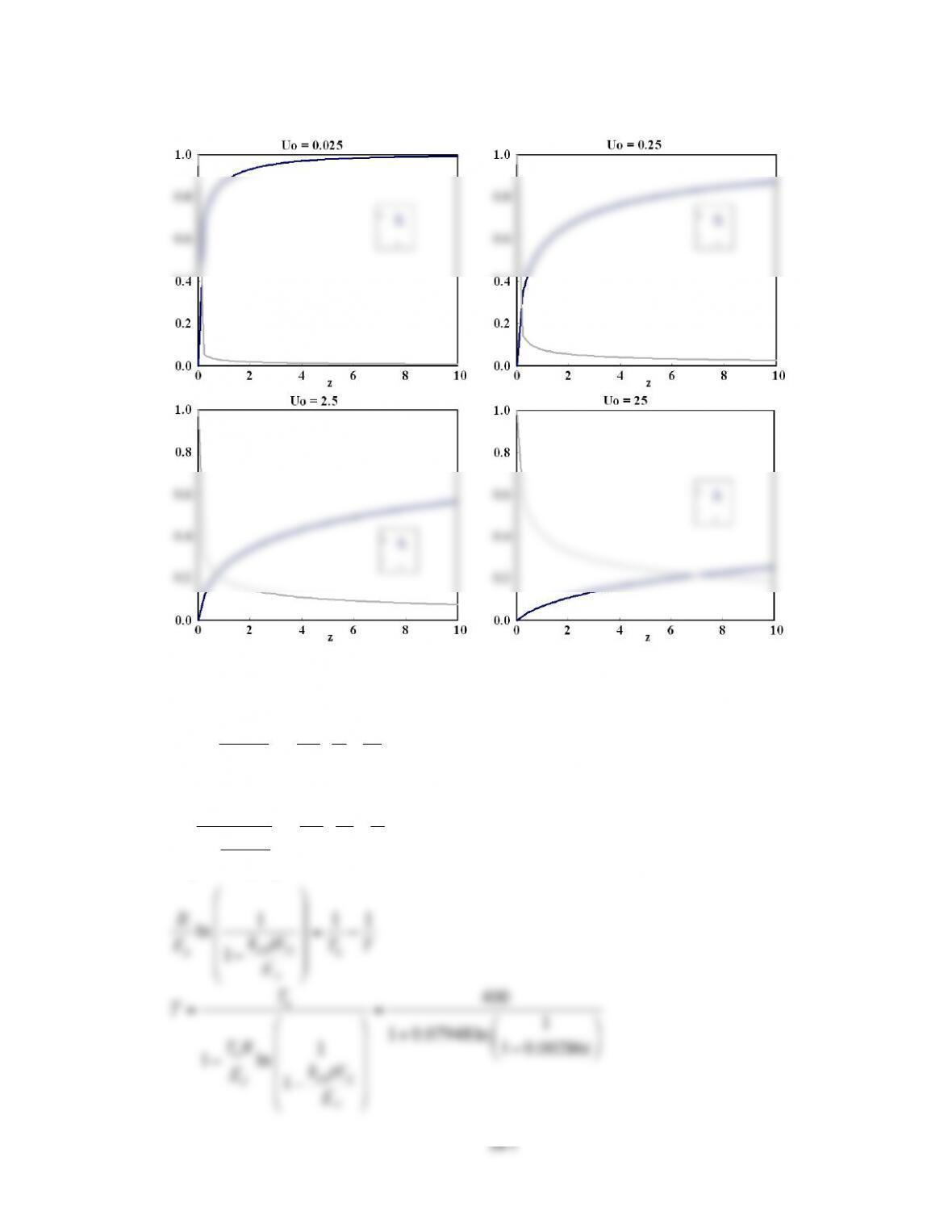
P10-2 (f) Example 10-6
Increasing the space time makes the minimum disappear. Decreasing the space time
moves the minimum to the left and the concentration is higher.
10-6
P10-2 (g) Example 10-7
(1) If the solids and reactants are fed from opposite ends,
d
S
k a
da
dW U
=
at W = We, a = 1
1
ln d
S
k
a W C
U
= +
1
d e
S
k W
C
U
=
( )
exp d
e
S
k
a W W
U
! “
=#
$ %
& ‘
( )2
2
0 0 1
A A
dX
F kC X a
dW =!
2
0
00
exp exp
1
We
A d e S d
A S d S
kC k W U k W
X
X F U k U
! “ ! “
#
=$ % $ %
#& ‘ & ‘
2
0
0
1 exp
1
A S d e
d A S
kC U k W
X
X k F U
! “
# $
%
=%
& ‘
( )
& ‘
%* +
, –
This gives the same expression for conversion as in the example.
(2) Second order decay
1
1d
S
ak W
U
=
+
2
0
0
ln 1
1
A S d
d A S
kC U k W
X
X k F U
! “
= +
# $
%& ‘
( )( )
( )( )
( )
2
0.6 0.075 0.72 22000
1.24 ln 1
0.72 30
S
S
U
U
! “
= +
# $
% &
Solve for US by trial and error or a non-linear equation solver.
US = 0.902
(3) If ε = 2
( )
( )
2
2
0 0 2
1
1
A A
X
dX
F kC a
dW X
!
“
=
+
( ) ( ) ( )22
20
0
1
2 1 ln 1 1 exp
1
A S d e
d A S
XkC U k W
X X
X k F U
!
! ! !
” #
+$ %
&
+&+ + = &
‘ (
) *
‘ (
&+ ,
– .
( ) 9
12 ln 1 4 1.24
1
X
X X
X
!+ + =
!
X = 0.372
10-7
P10-2 (h) Example 10-8
P10-2 (i)
For EA = 10 and Ed = 35, for first order decay we rearrange Eq 10-120 to:
0
0
1 1
ln 1 d d d
A
k tE E
E R T T
! “
! “
#=#
$ %
$ %
& ‘ & ‘
00
1 1 1
ln
1
d
d d
A
E
k tE R T T
E
! “
# $ ! “
# $ =%
# $
# $ & ‘
%
# $
& ‘
00
1 1 1
ln
1d d
d
A
R
k tE
E T T
E
! “
# $
# $ =%
# $
%
# $
& ‘
0
0
0
400
1
1 0.07948 ln
1 0.00286
1
1 ln
1d d
d
A
T
T
t
T R
k tE
E
E
= =
! “ ! “
+# $
# $ %
& ‘
# $
%# $
%
# $
& ‘
10-8
P10-2 (j) Individualized solution
P10-3 Solution is in the decoding algorithm given with the modules
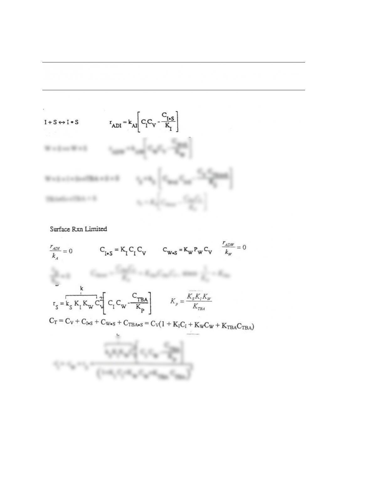
P10-4
P10-4 (a)
10-9
P10-4 (b)
Adsorption of isobutene limited
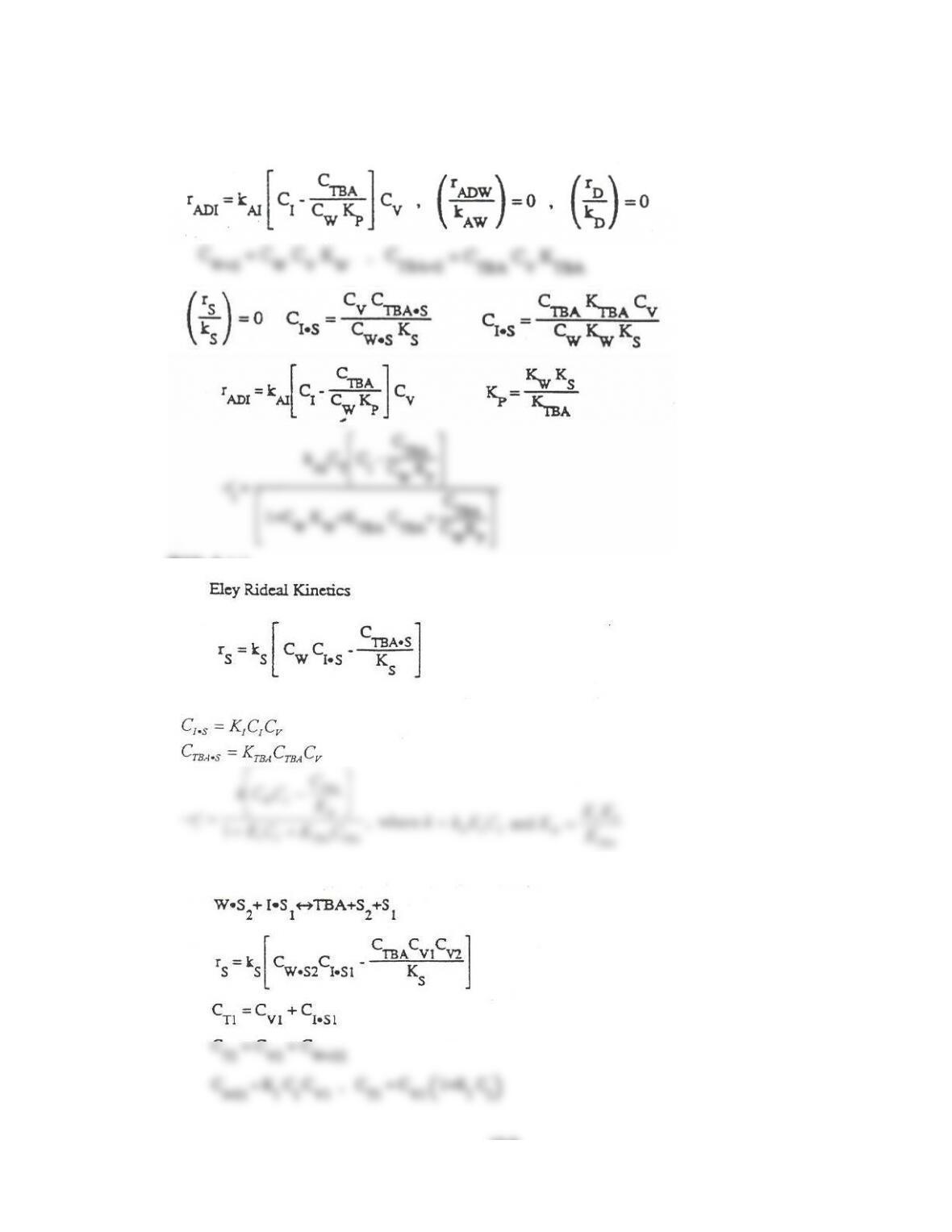
P10-4 (d)
10-10
P10-4 (e) Individualized solution
P10-4 (f) Individualized solution
P10-5 (a)
P10-5 (b) Individualized solution
P10-5 (c)
22 2O S O S
!!“
+ •
#!!
22 2A S A S
!!“
+ •
#!!
3 6 3 5
C H O S C H OH S+ • !•
B A S C S+ • !•
3 6 3 5
C H OH S C H OH S
!!“
• +
#!!
C S C S•!+
3B S B A S
r r k P C •
!= =
2
2
2A S
AD A A V
A
C
r k P C
K
•
! “
=#
$ %
& ‘
0
AD
A
r
k=
A S V A A
C C K P=
3B S B V A A
r r k P C K P!= =
10-11
[ ]
C V
C S D C S D C S C C V
D
P C
r k C k C K P C
K
• • •
! “
=#=#
$ %
& ‘
0
C S
r
k
•=
P10-6 (a)
10-12
P10-6 (b)
P10-6 (c)
10-13
P10-6 (d) Individualized solution
P10-6 (e) Individualized solution
P10-7
10-14
P10-8
P10-8 (a)
10-15
P10-8 (b)
P10-8 (c)
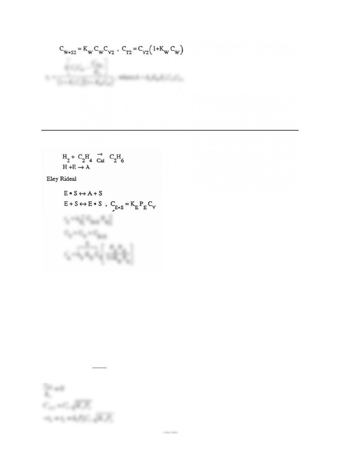
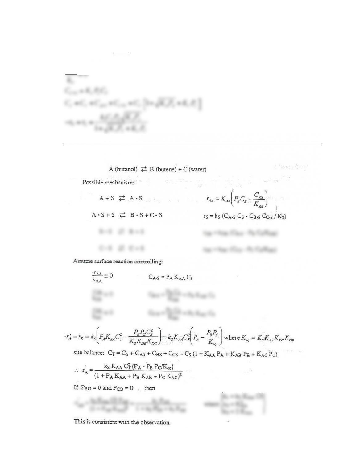
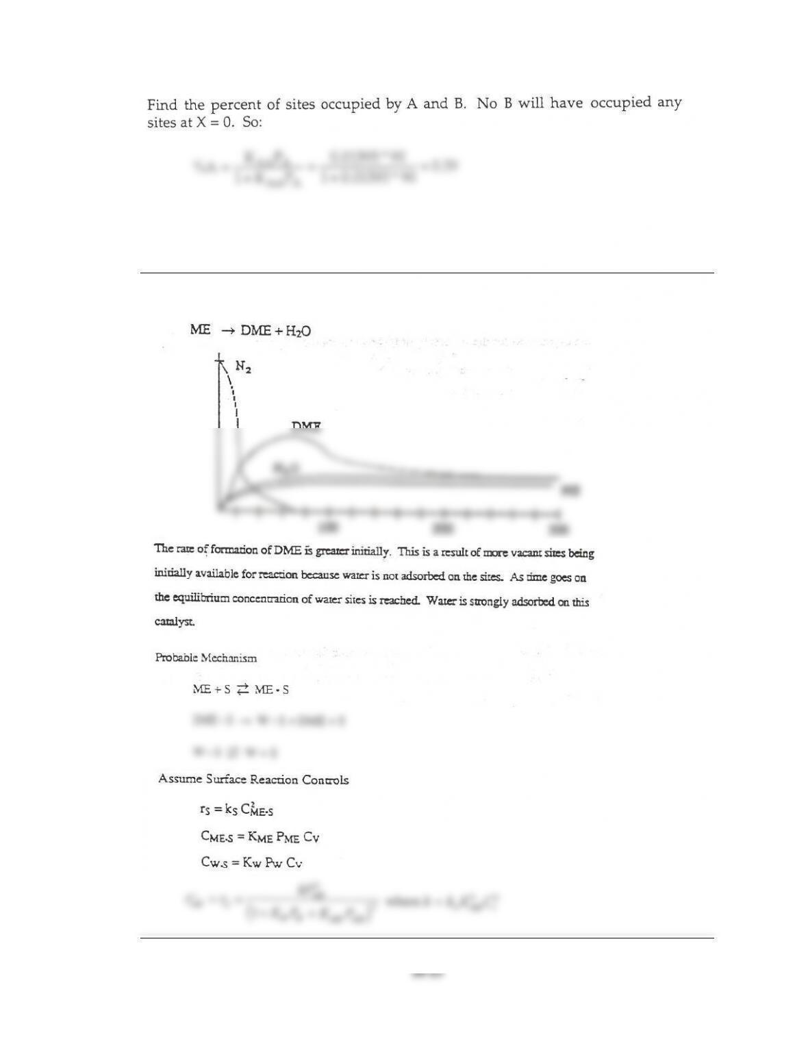
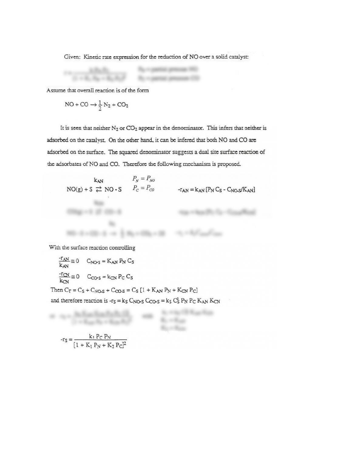
P10-9
10-16
P10-9 (a)
10-17
P10-9 (b)
10-18
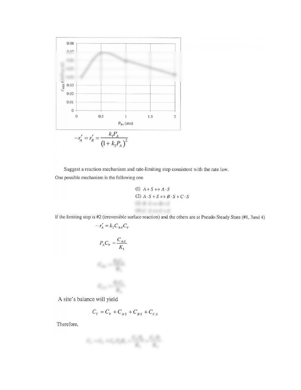
Substituting the expressions for CV and CA·S into the equation for –r’A
P10-9 (c) Individualized solution
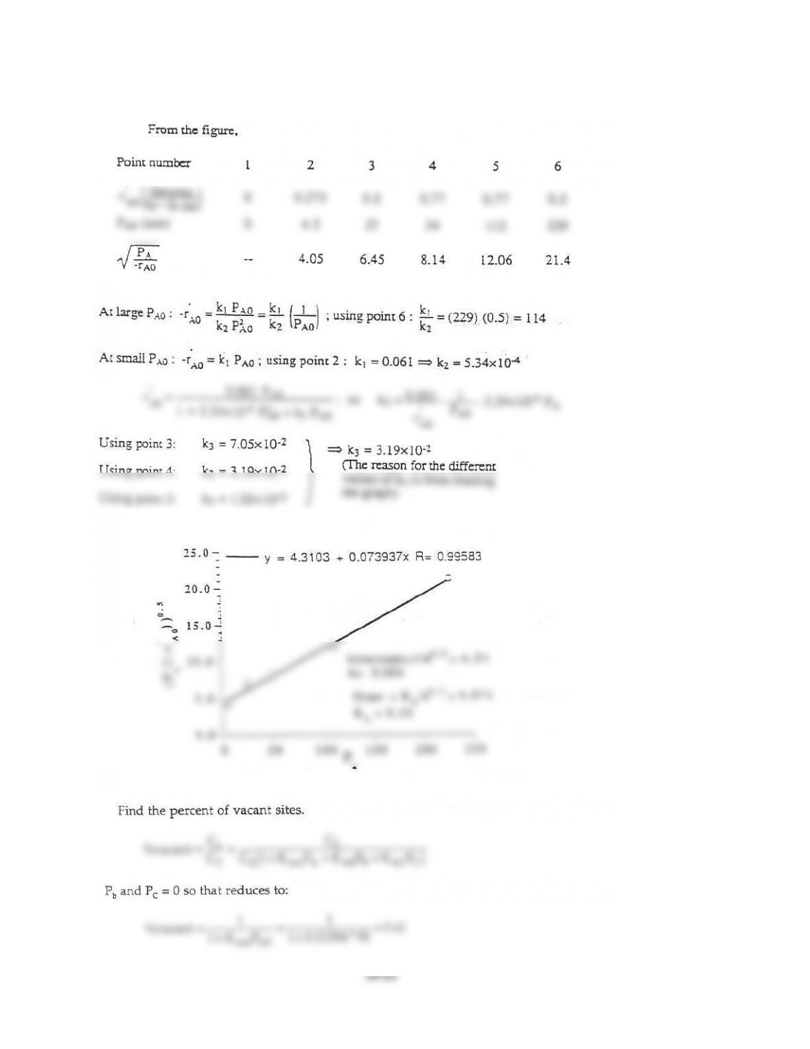
P10-9 (d)
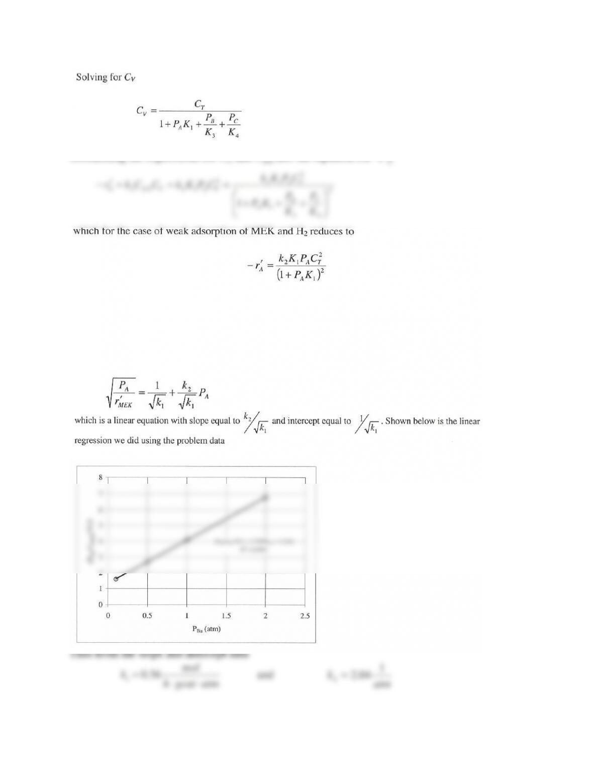
First we need to calculate the rate constants involved in the equation
for –r’A in part (a). We can rearrange the equation to give the
following
Thus from the slope and intercept data
10-19
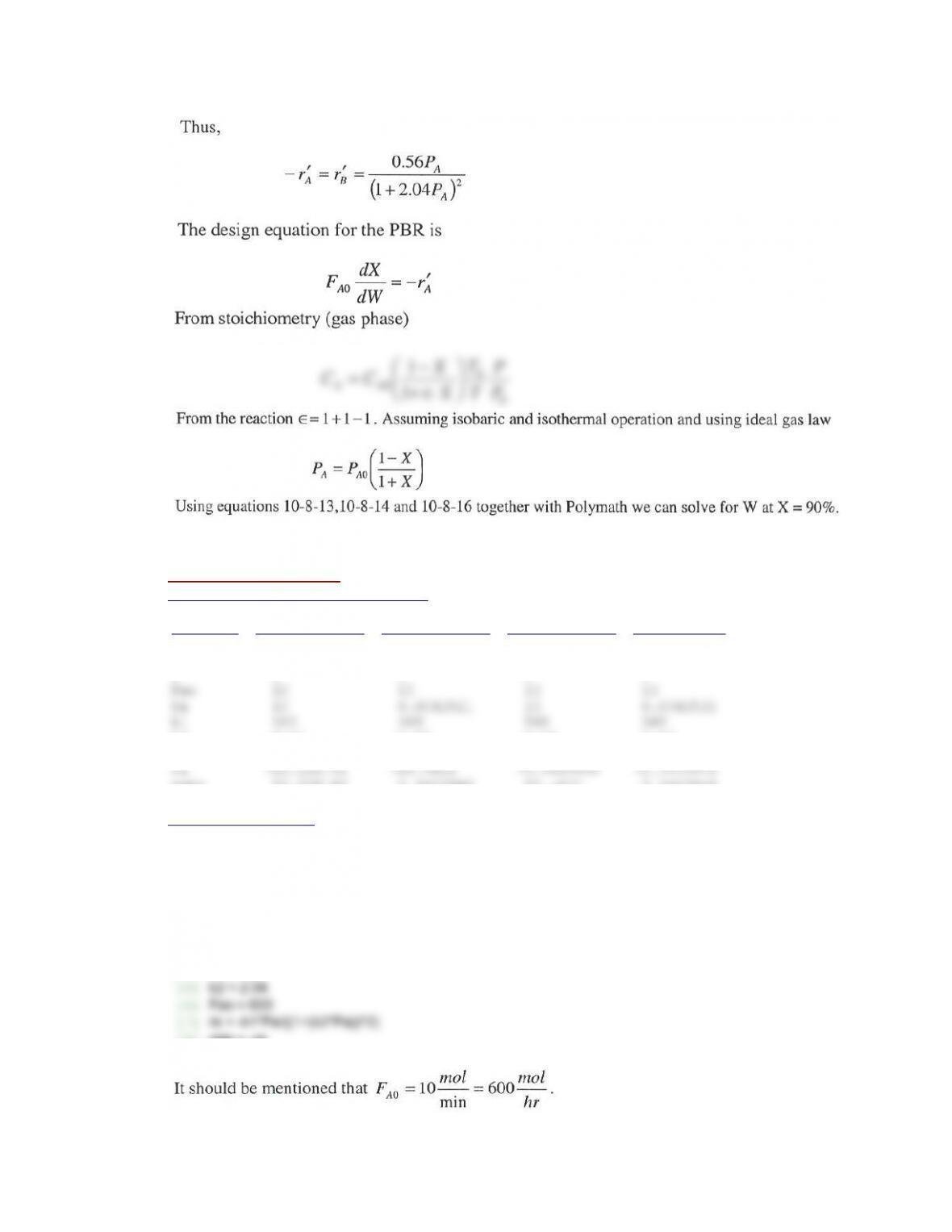
See Polymath program P10-9-d.pol.
POLYMATH Results
Calculated values of the DEQ variables
Variable initial value minimal value maximal value final value
W 0 0 23 23
X 0 0 0.9991499 0.9991499
e 1 1 1 1
Pao 10 10 10 10
Fao 600 600 600 600
ra -12.228142 -68.5622 –2.3403948 -2.3403948
ODE Report (RKF45)
Differential equations as entered by the user
[1] d(X)/d(W) = -ra/Fao
Explicit equations as entered by the user
[1] e = 1
[2] Pao = 10
[3] Pa = Pao*(1-X)/(1+e*X)
[4] k1 = 560
[5] k2 = 2.04
10-20
P10-9 (e) Individualized solution
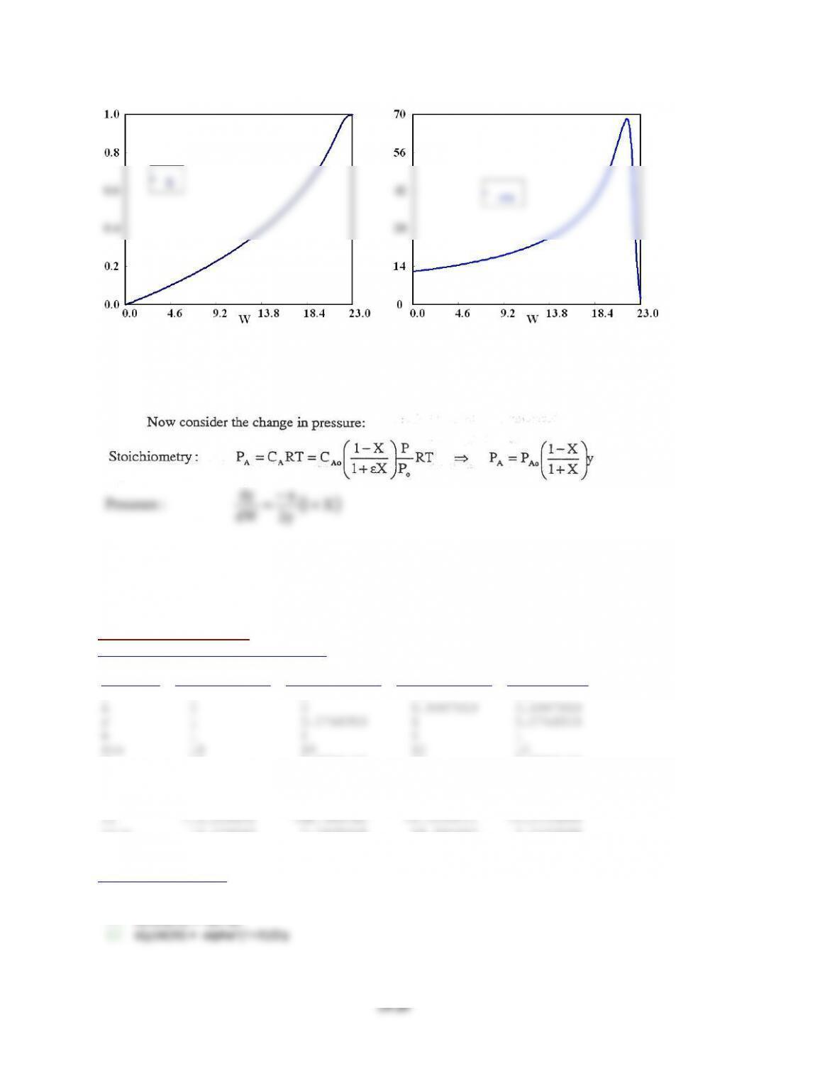
P10-9 (f)
Use these new equations in the Polymath program from part (d).
See Polymath program P10-9-f.pol.
POLYMATH Results
Calculated values of the DEQ variables
Variable initial value minimal value maximal value final value
W 0 0 23 23
X 0 0 0.9997919 0.9997919
k1 560 560 560 560
k2 2.04 2.04 2.04 2.04
Fao 600 600 600 600
ra -12.228142 -68.584462 –0.0435044 -0.0435044
alpha 0.03 0.03 0.03 0.03
ODE Report (RKF45)
Differential equations as entered by the user
[1] d(X)/d(W) = -ra/Fao
[2] d(y)/d(W) = -alpha*(1+X)/2/y