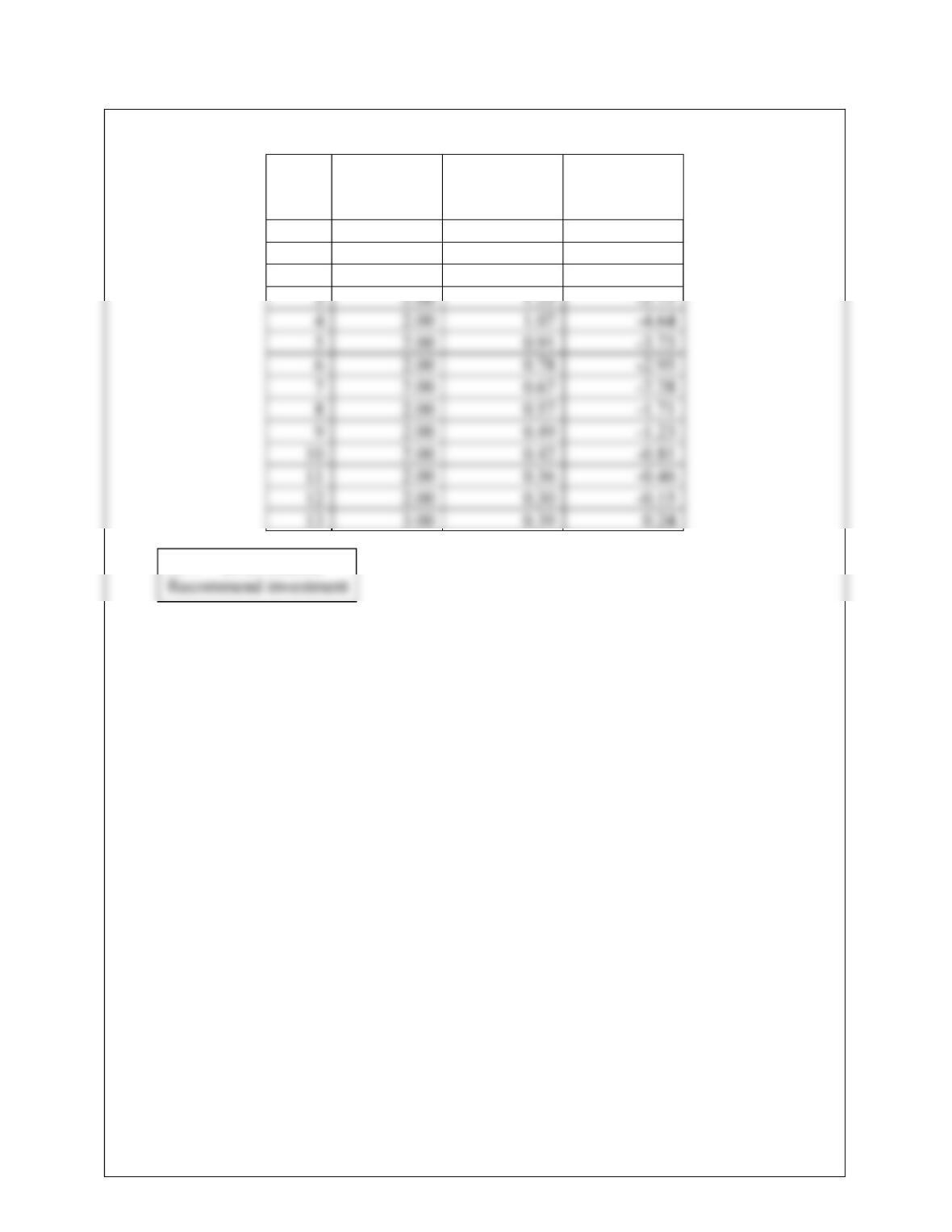
10-19
10.25 Look at incremental cases.
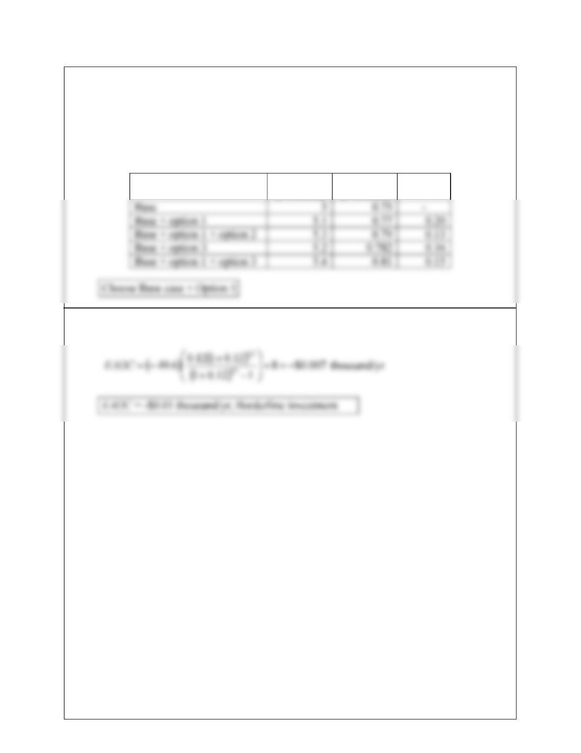
ROROII = Incremental Yearly Savings / Incremental Investment
ROROIIBase +1 – Base = (0.77-0.75)/(5.1-5) = 0.20
See table for complete ROROII calculations.
Case FCI
($ million)
Cash Flow
($ million) ROROII
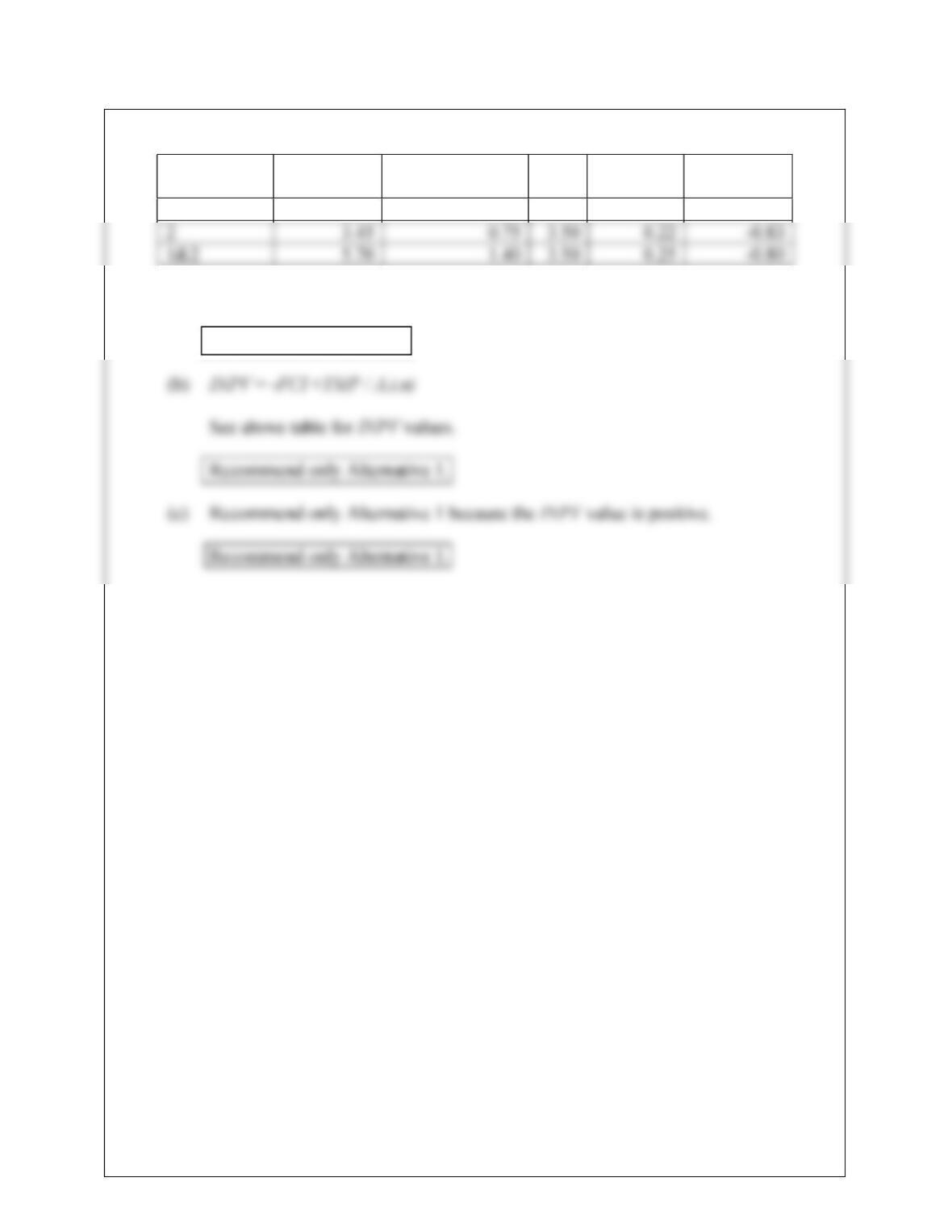
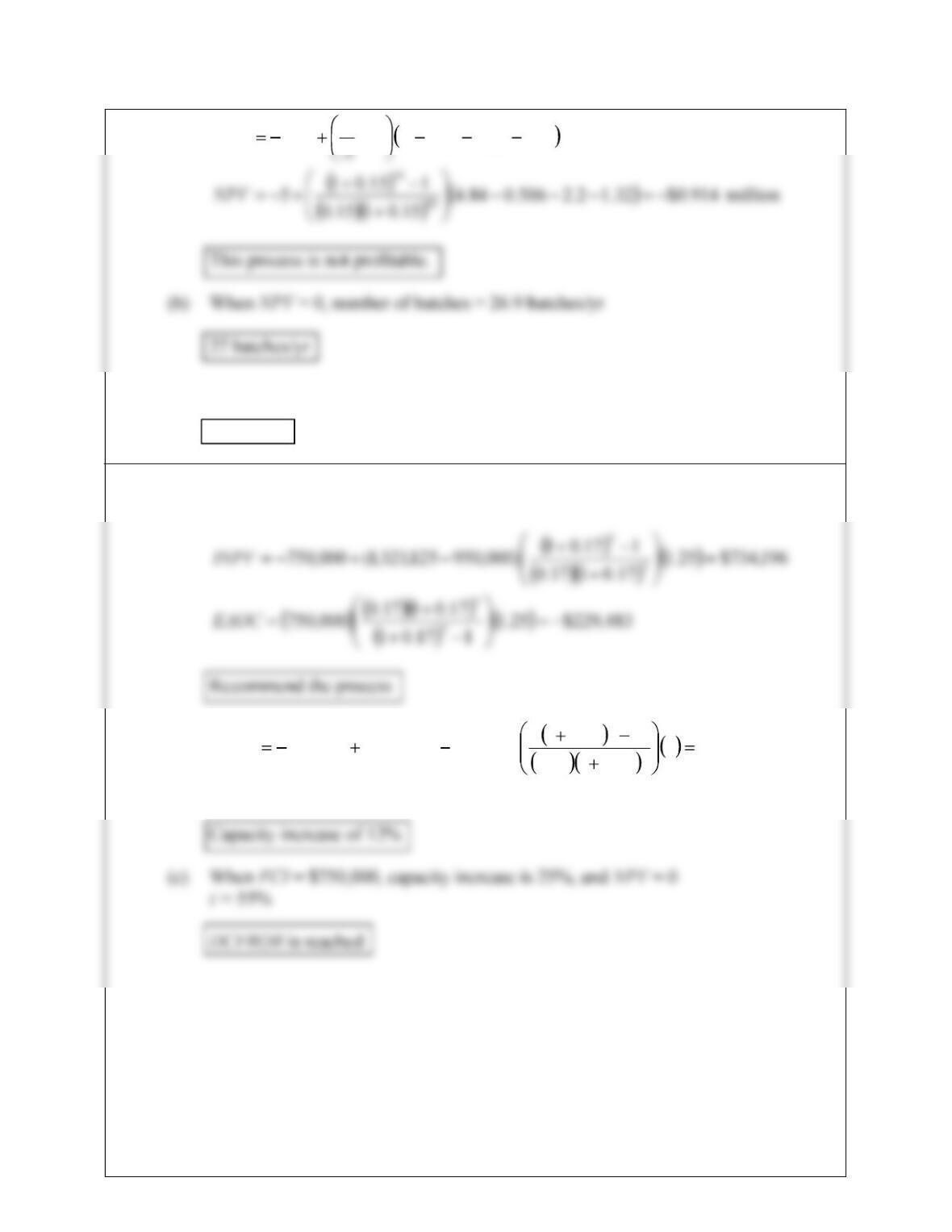
10.26 EAOC = -FCI(A/P,i,n) +YS
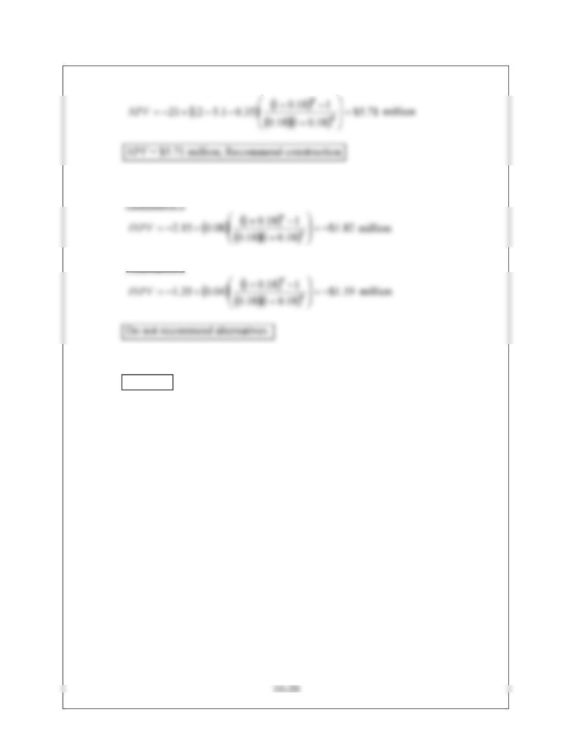
10.27 (a) Base Case
NPV = –FCI +CFi(P / A,i,n)
(b) INPV = –FCI +YS(P / A,i,n)
Alternative 2
(c) INPV = 0 = -3.26+4.08YS
YS = 0.80
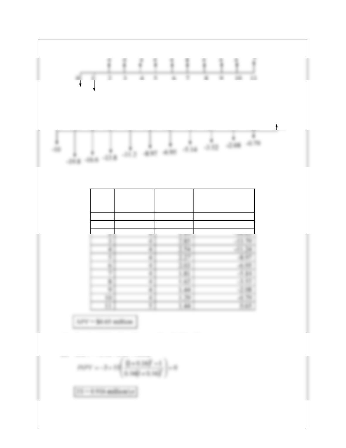
10-21
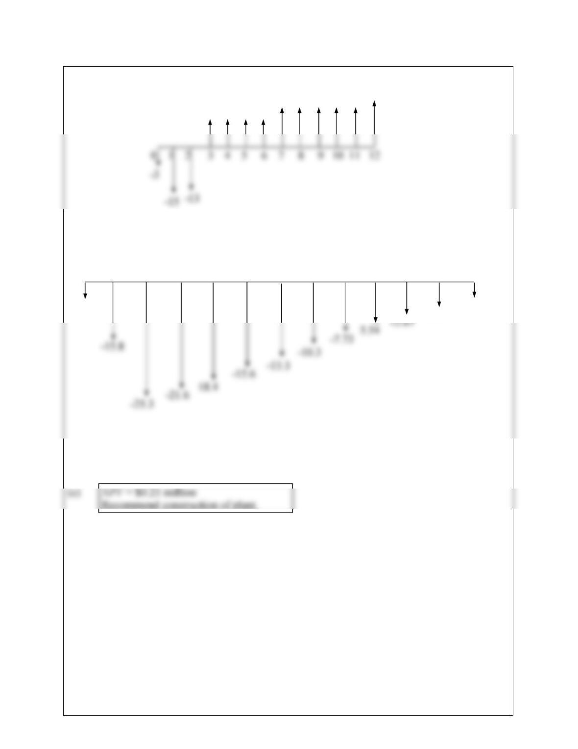
10.28 (a) All values are in $ millions.
(b) All values are in $ millions.
6 6 6 6
9 9 9 9 9 15
0 1 2 3 4 5 6 7 8 9 10 11 12
-3
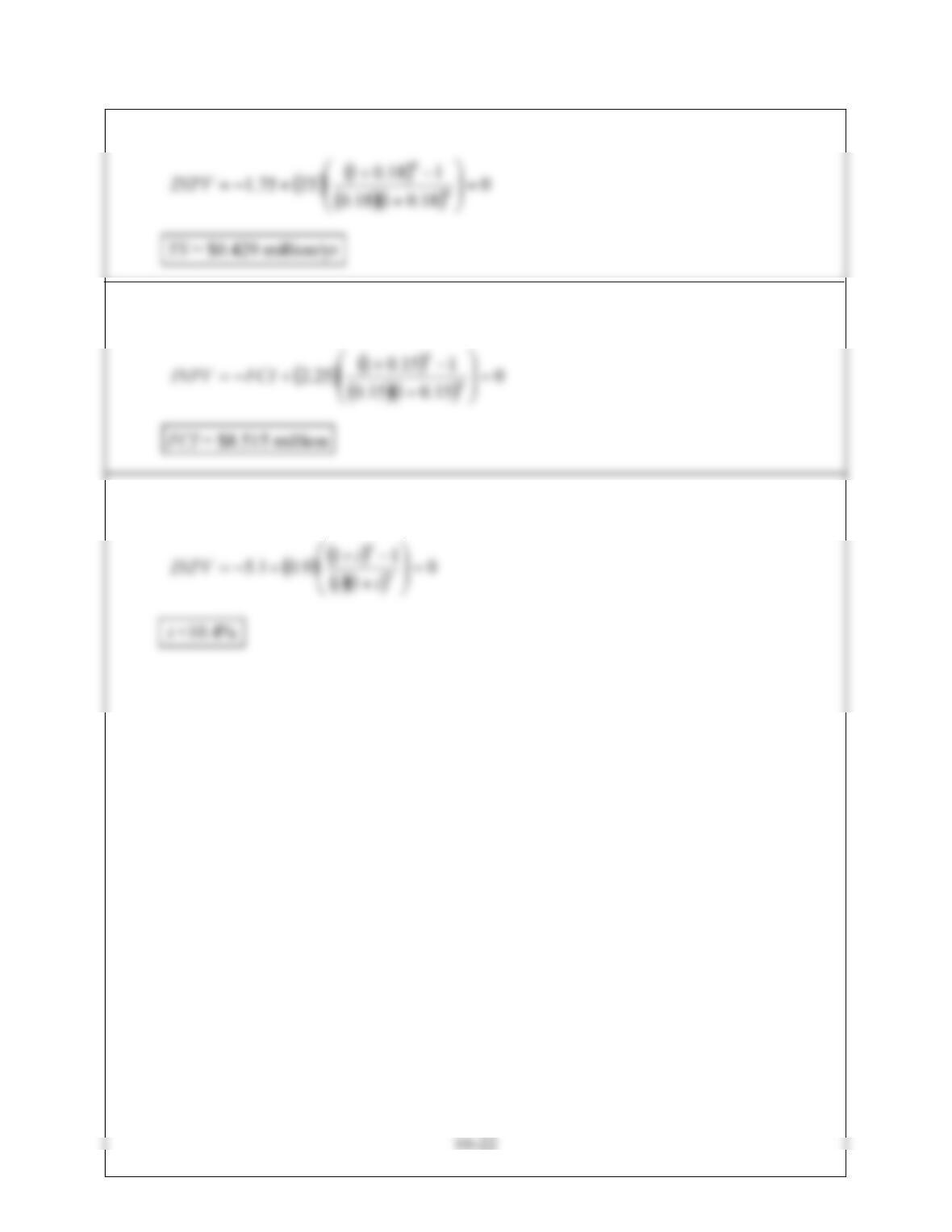
10.29 INPV = –FCI +YS(P / A,i,n)
10.30 INPV = –FCI +YS(P / A,i,n)
10.31 INPV = –FCI +YS(P / A,i,n)
10-23
10.32
Year Cash Flow
($ million)
Discounted
Case Flow
($ million)
Cumulative
Cash Flow
($ million)
0 -5.00 -5.00 -5.00
1 -4.00 -3.42 -8.42
2 2.00 1.46 -6.96
NPV = $0.24 million
10-24
10.33 (a) ROROII = Incremental Yearly Savings / Incremental Investment
Alternative FCI
($ million)
Yearly Savings
($ million) P/A ROROII INPV
($ million)
1 2.25 0.65 3.50 0.29 0.02
All ROROII values are greater than 18%; therefore, all alternatives are good.
All alternatives will work.
10-25
10.34 (a) All values are in $ millions.
(b) All values are in $ millions.
(c)
Year Cash Flow
($ million)
Discounted
Cash Flow
($ million)
Cumulative Disc.
Cash Flow
($ million)
0 -10 -10.00 -10.00
1 -11 -9.82 -19.82
(d) For the NPV = $2 million, profit = $4.27 million
(e) INPV = –FCI +YS(P / A,i,n)
-10 -11
0 1 2 3 4 5 6 7 8 9 10 11
0.65
10.35 EAOC = FCI(A/P,i,n) + YOC
65.7$5.5
114.01
14.0114.0
53
3
A
EAOC thousand/yr
10.36 EAOC = FCI(A/P,i,n) – YS
39.53$332515
115.01
15.0115.0
88 8
8
A
EAOC thousand/yr
10-27
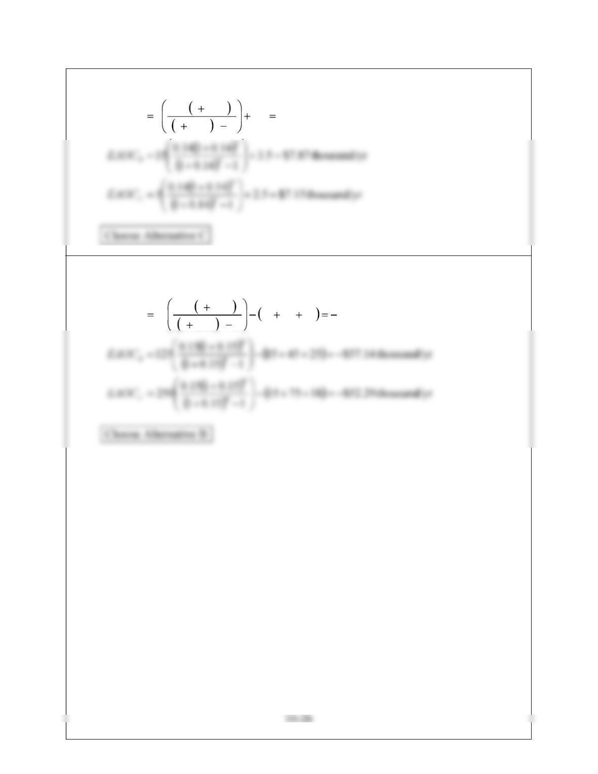
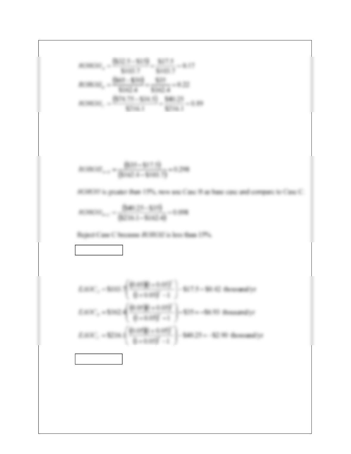
10.37 (a) ROROII = Incremental Yearly Savings / Incremental Investment
From above, choose Case B. However, can also do incremental comparison
between cases.
Use Case A as base case because it has the lowest FCI and evaluate ROROII going
from Case A to Case B.
Choose Case B
(b) EAOC = FCI(A/P,i,n) – YS
Choose Case B
10-28
(c) EAOC = FCI(A/P,i,n) – YS
Choose Case C
(d) EAOC = FCI(A/P,i,n) – YS
None of the cases provide an acceptable EAOC.
10-29
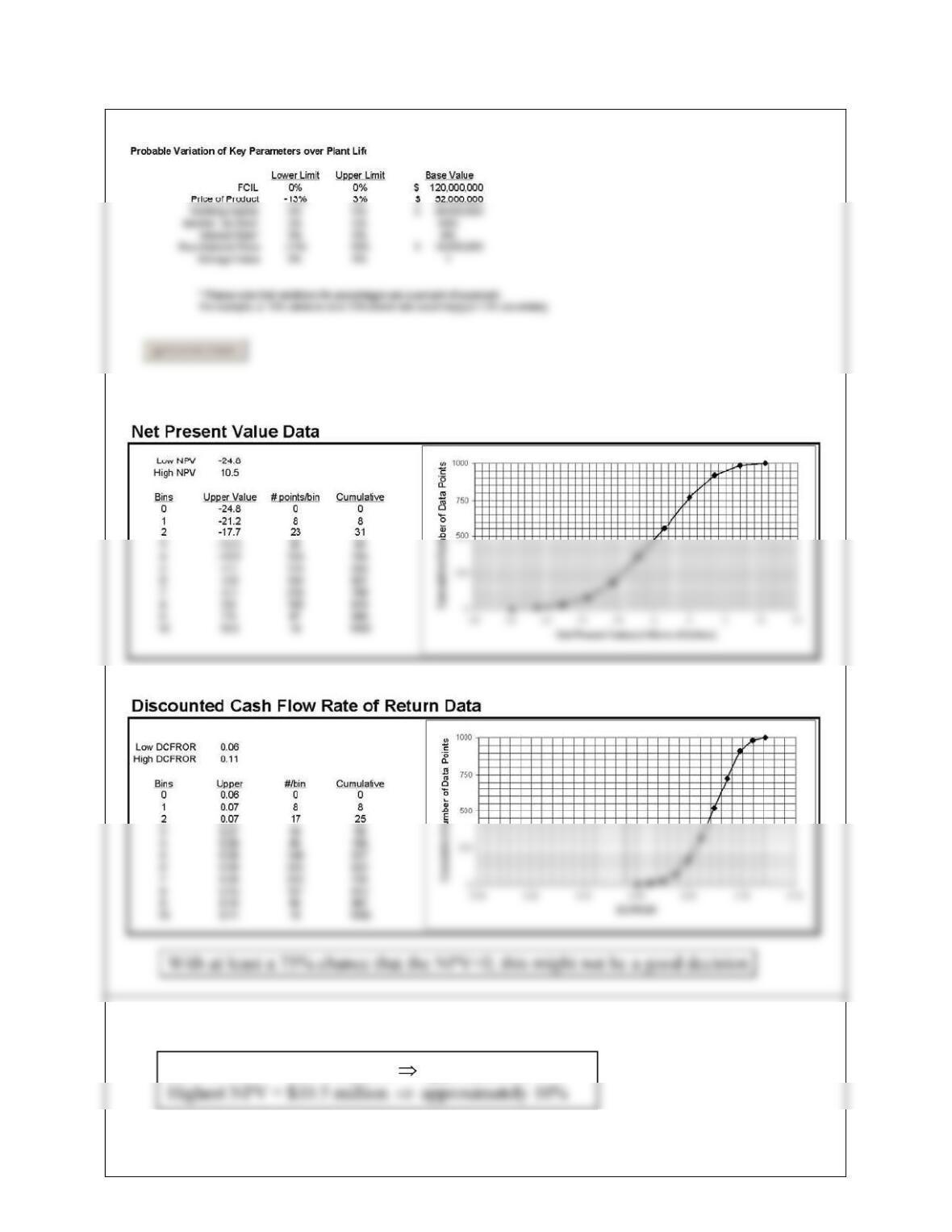
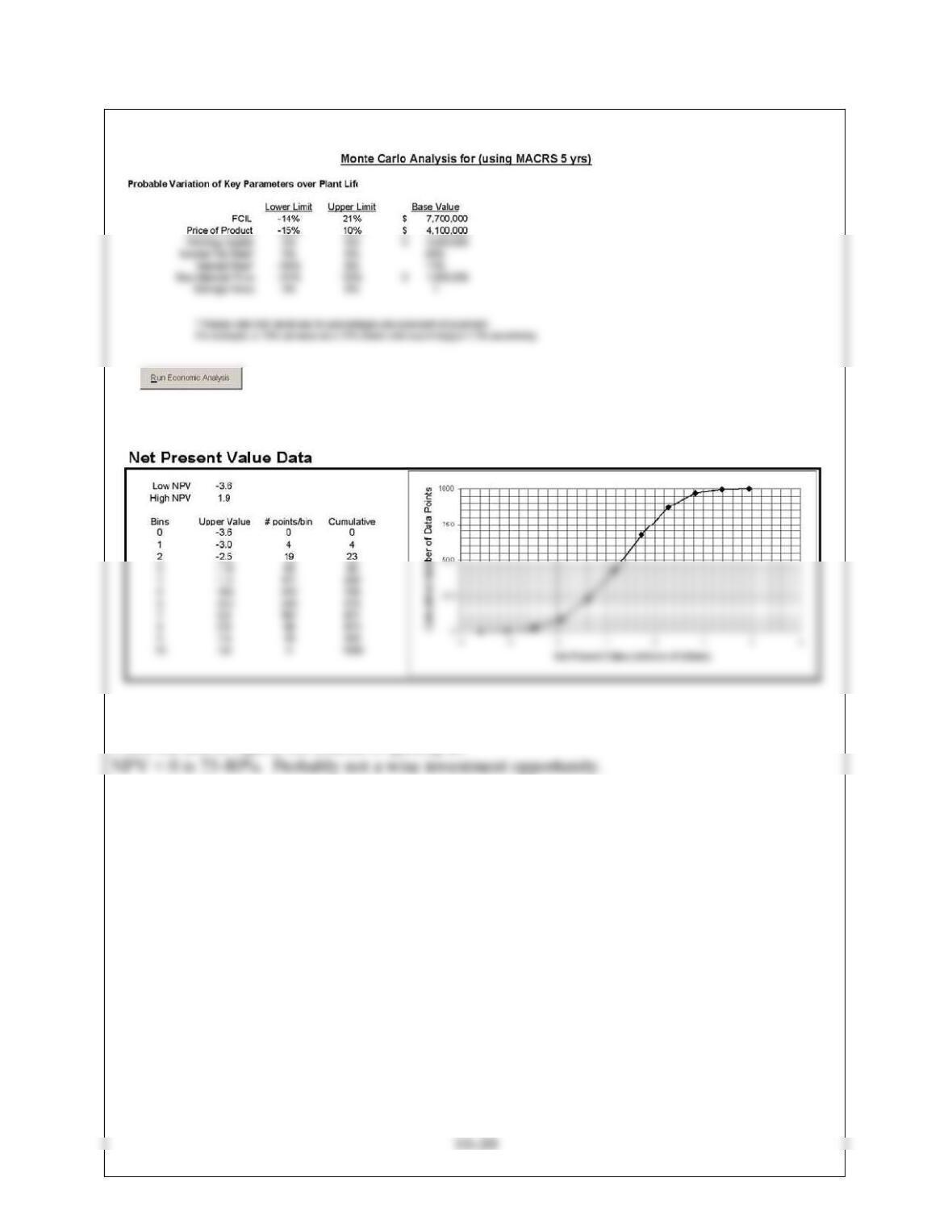
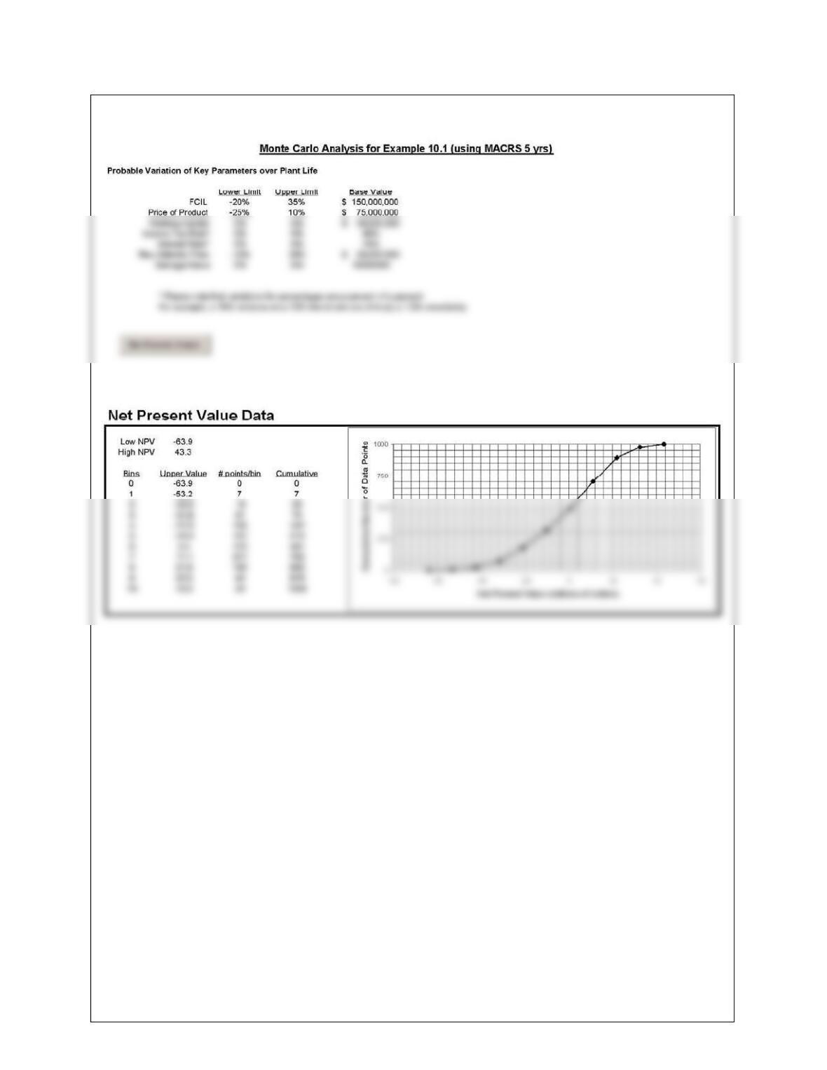
10.38 Individual solutions may differ slightly because of the Monte Carlo method being used.
10.39
Lowest NPV = -$24.8 million approximately 1%
10.40
From the above figure, the chance of getting an
10-31
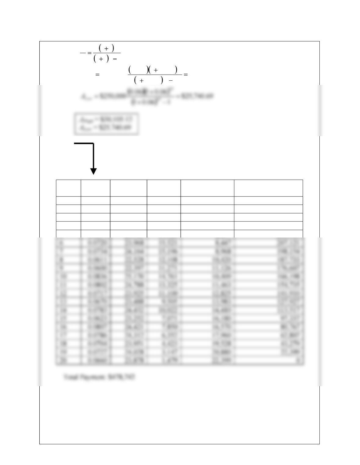
10.41 (a) 11
1
n
n
i
ii
P
A
12.105,30$
1085.01
085.01085.0
000,250$ 15
15
High
A
(b)
(c)
Variable Rate Simulation
Year iPayment
($/y)
Interest
($/y)
Principal Paid
($/y)
Remaining Balance
($/y)
1 0.0765 24,795 19,114 5,681 244,319
2 0.0664 23,010 16,230 6,779 237,539
3 0.0727 24,078 17,271 6,807 230,732
4 0.0757 24,577 17,471 7,106 223,626
5 0.0694 23,583 15,526 8,057 215,569
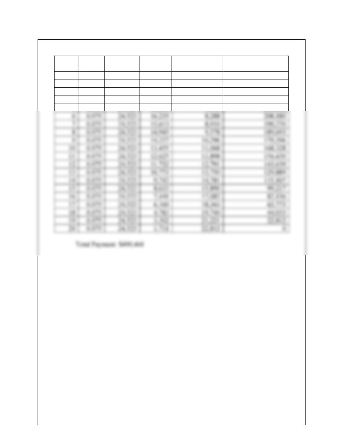
10-32
Fixed Rate Simulation
Year iPayment
($/y)
Interest
($/y)
Principal Paid
($/y)
Remaining Balance
($/y)
1 0.075 24,523 18,750 5,773 244,227
2 0.075 24,523 18,317 6,206 238,021
3 0.075 24,523 17,852 6,671 231,349
4 0.075 24,523 17,351 7,172 224,178
5 0.075 24,523 16,813 7,710 216,468
10-33
10.42
10-34
10.43 (a) UTRMWT CCCRni
P
FCINPV ,,
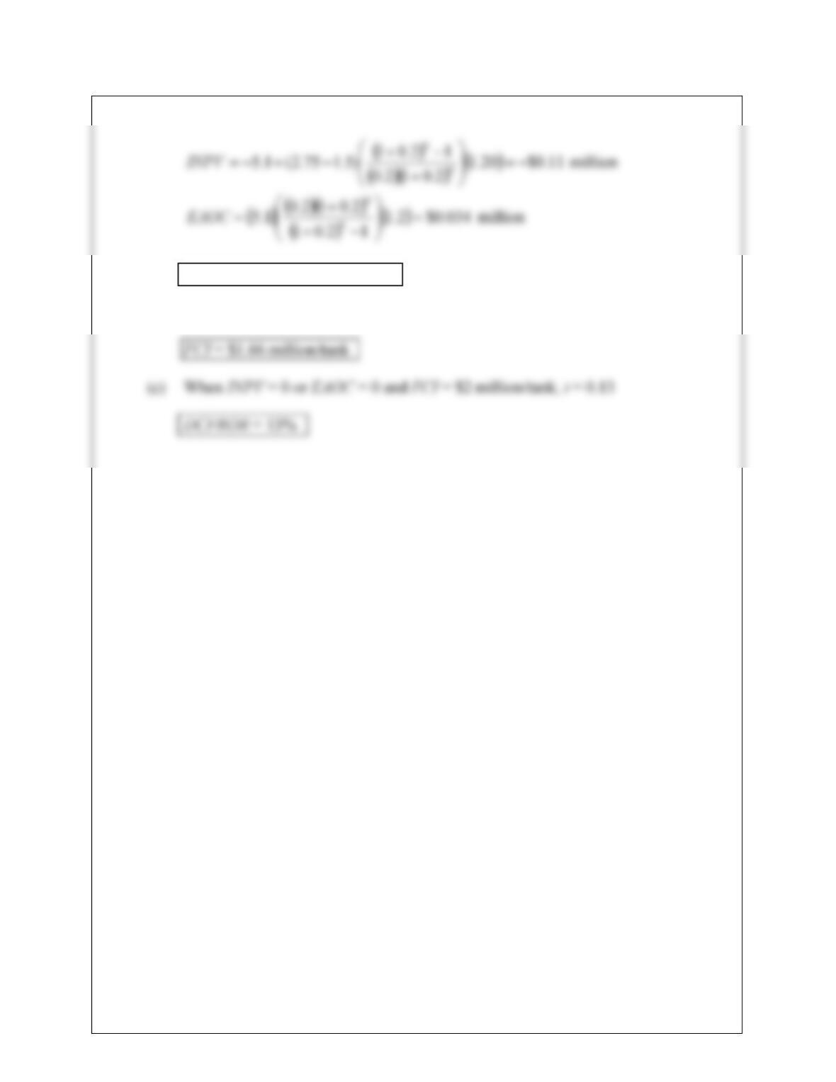
(c) When NPV = 0 and number of batches = 26/yr, i = 14.1%
i = 14.1%
10.44 (a) INPV = –FCI +YS(P / A,i,n) or EAOC = FCI(A/P,i,n) – YS
(b) 196,734$
17.0117.0
117.01
)000,950125,321,1(000,750 5
5
xINPV
x = 1.12
10-35
10.45 (a) INPV = –FCI +YS(P / A,i,n) or EAOC = FCI(A/P,i,n) – YS
Do not recommend this process.
(b) When INPV = 0 or EAOC = 0, FCI = $4.99 million