Time Rate of Consolidation Chapter 9
CHAPTER 9
TIME RATE OF CONSOLIDATION
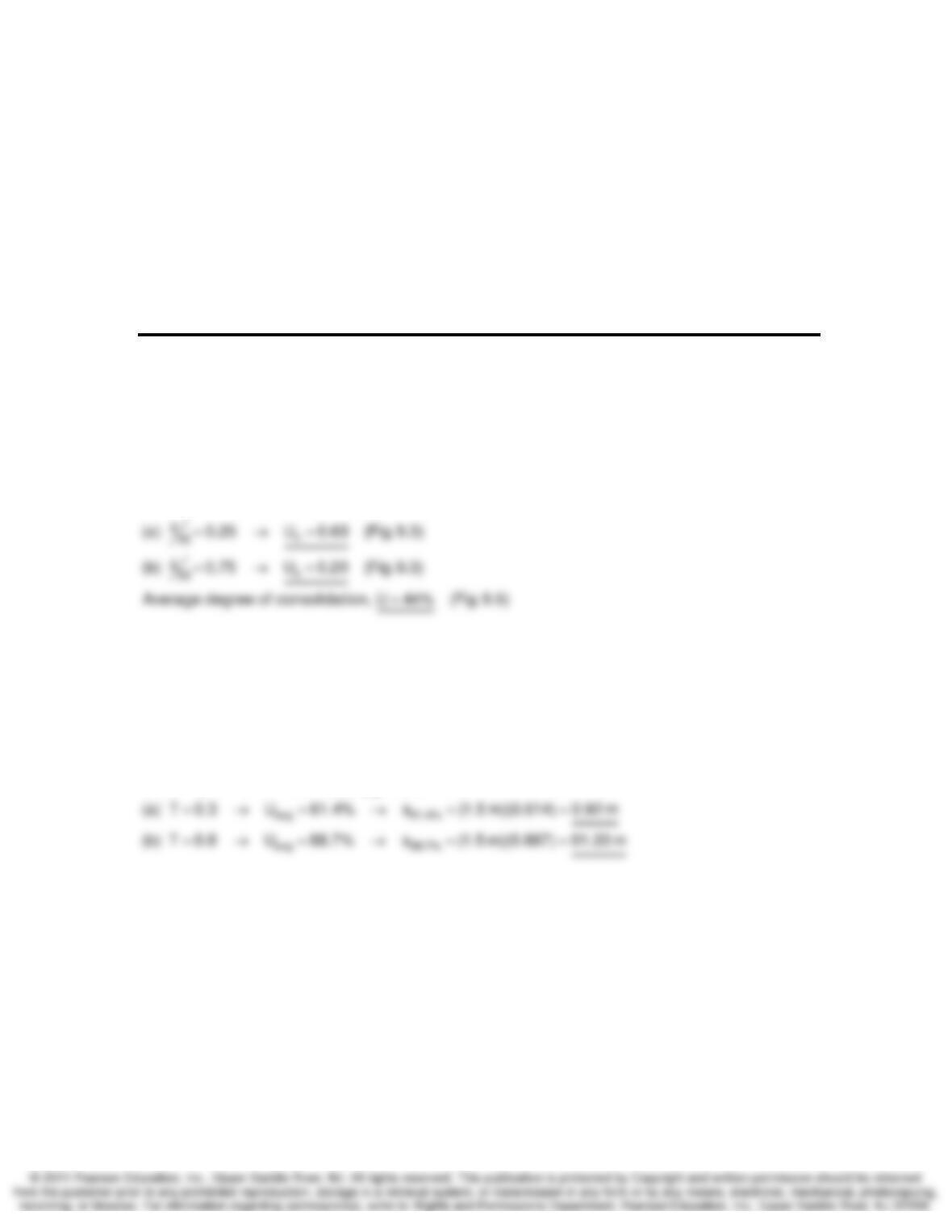
9-1. The time factor for a clay layer undergoing consolidation is 0.15. What is the degree of
consolidation (consolidation ratio) at the center and at the quarter points (that is, z/H = 0.25 and
0.75)? What is the average degree of consolidation for the layer?
SOLUTION:
T0.15
=
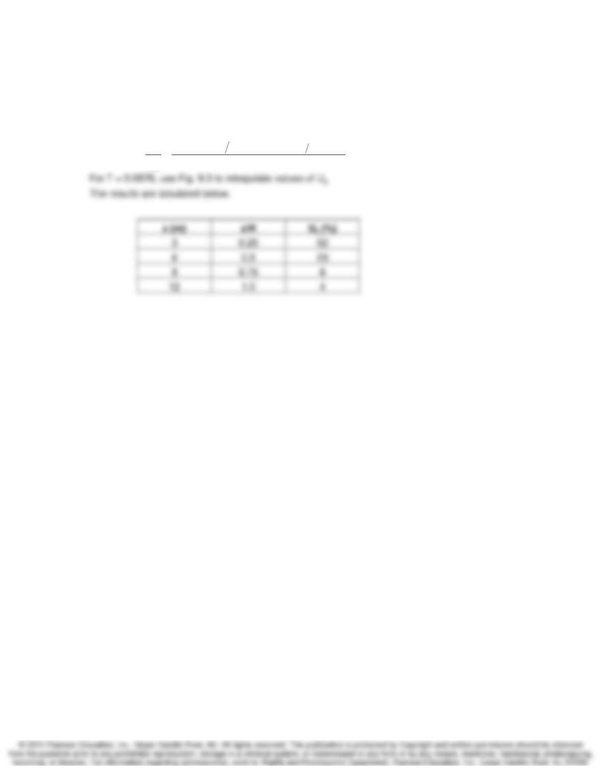
9-2. If the final consolidation settlement for the clay layer of Problem 9.1 is expected to be 1.5 m,
how much settlement has occurred when the time factor is (a) 0.3 and (b) 0.8?
SOLUTION:
ccavg
Given: s 1.5 m : s(t) (s )U (Eq. 9.12)
==
Time Rate of Consolidation Chapter 9
9-3. If the clay layer of Example 9.1 were singly drained, would there be any difference in the
calculated values? If so, how much difference?
SOLUTION:
dr
82 7
v
22
dr
Yes, H 12 m for single layer
ct (8.0)(10 m s )(3.1536)(10 s yr)(5 yr)
Eq. 9.5: T 0.0876 (compares to 0.35 in Ex. 9.1)
H(12m)
−
=
== =
Time Rate of Consolidation Chapter 9
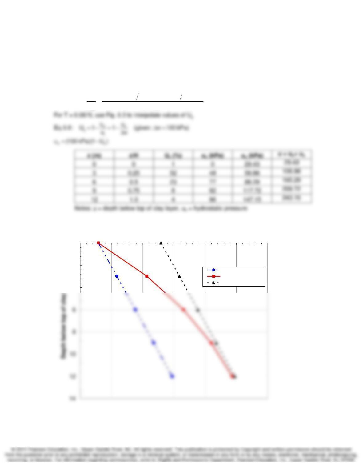
9-4. Plot a graph of excess pore pressure versus depth, similar to Fig. Ex. 9.2, for the soil and
loading conditions given in Example 9.2, but for the case of single drainage. Assume that under
the clay there is impervious shale instead of a dense sand.
SOLUTION:
dr
82 7
v
22
dr
H 12 m for single layer
ct (8.0)(10 m s)(3.1536)(10 s yr)(5 yr)
Eq. 9.5: T 0.0876 (compares to 0.35 in Ex. 9.1)
H(12m)
−
=
== =
0
2
4
0 50 100 150 200 250 300
u (kPa)
Hydrostatic pressure
Excess pore pressure
u = 100 kPa at t = 0
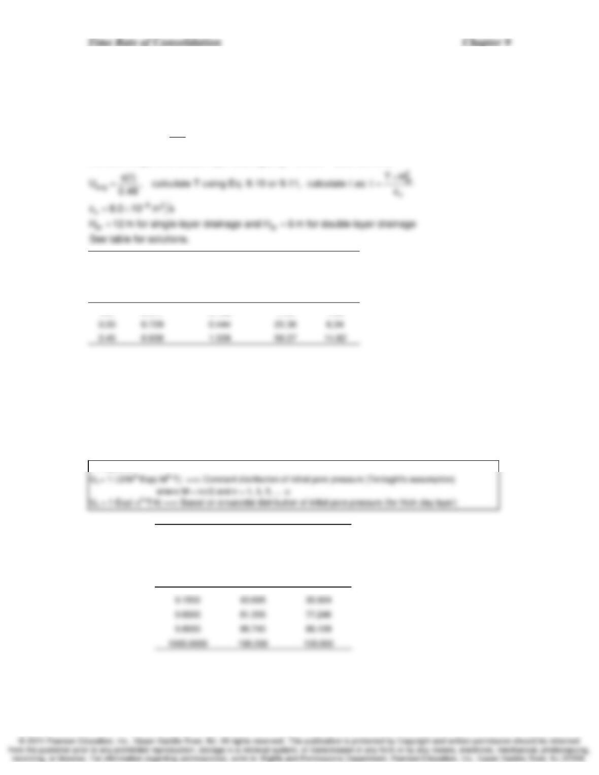
9-5. For the soil and loading conditions of Examples 9.1 and 9.2, estimate how long it would take
for 0.2, 0.35, and 0.45 m of settlement to occur. Consider both single and double drainage.
SOLUTION:
avg
c
c
s(t)
(Eq. 9.12): U s
For both single and double-layer drainage, s 0.48 m (see Ex. 9.5)
=
=
single
drainage
double
drainage
s(t) U
avg
Ttt
(m) (decimal) (Eq. 9.10 or 9.11) (yr) (yr)
0.2 0.417 0.136 7.78 1.95
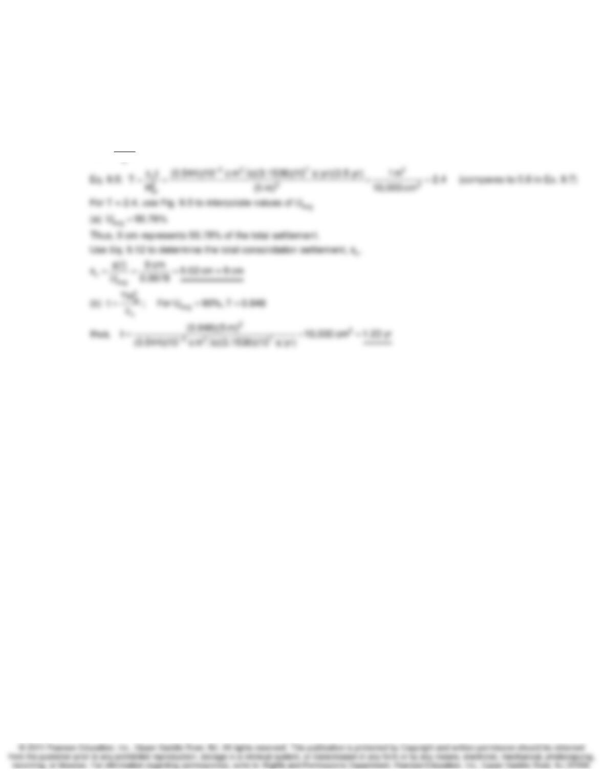
9-6. By evaluation of the series expression [Eq. (B.2.23) in Appendix B.2] for the solution to the
consolidation equation, determine the average degree of consolidation U to the nearest 0.001 for
time factors 0.15, 0.6, 0.8 and infinity. Verify your computations by referring to Table 9.1 and Fig.
9.5(a). Also check by Eqs. (9.10 and 9.11). (After Taylor, 1948.)
SOLUTION:
EQUATIONS
T = c
v
(t/D
2
)
2
2
2
(Constant u
i
)(Sinusoidal u
i
)(Sinusoidal u
i
)
Real Time Factor Degree of Degree of Settlement at
Time, t Consolidation Consolidation Time t
(yr) (%) (%) (in)
t TU
avg
U
s-avg
S
c
S
s
Time Rate of Consolidation Chapter 9
9-7. How much difference would there be in the (a) computed ultimate settlement and (b) the
time required for 90% consolidation for the soil conditions of Example 9.7 if the clay layer were
doubly drained?
SOLUTION:
dr
10 m
H 5 m for double-layer drainage
==
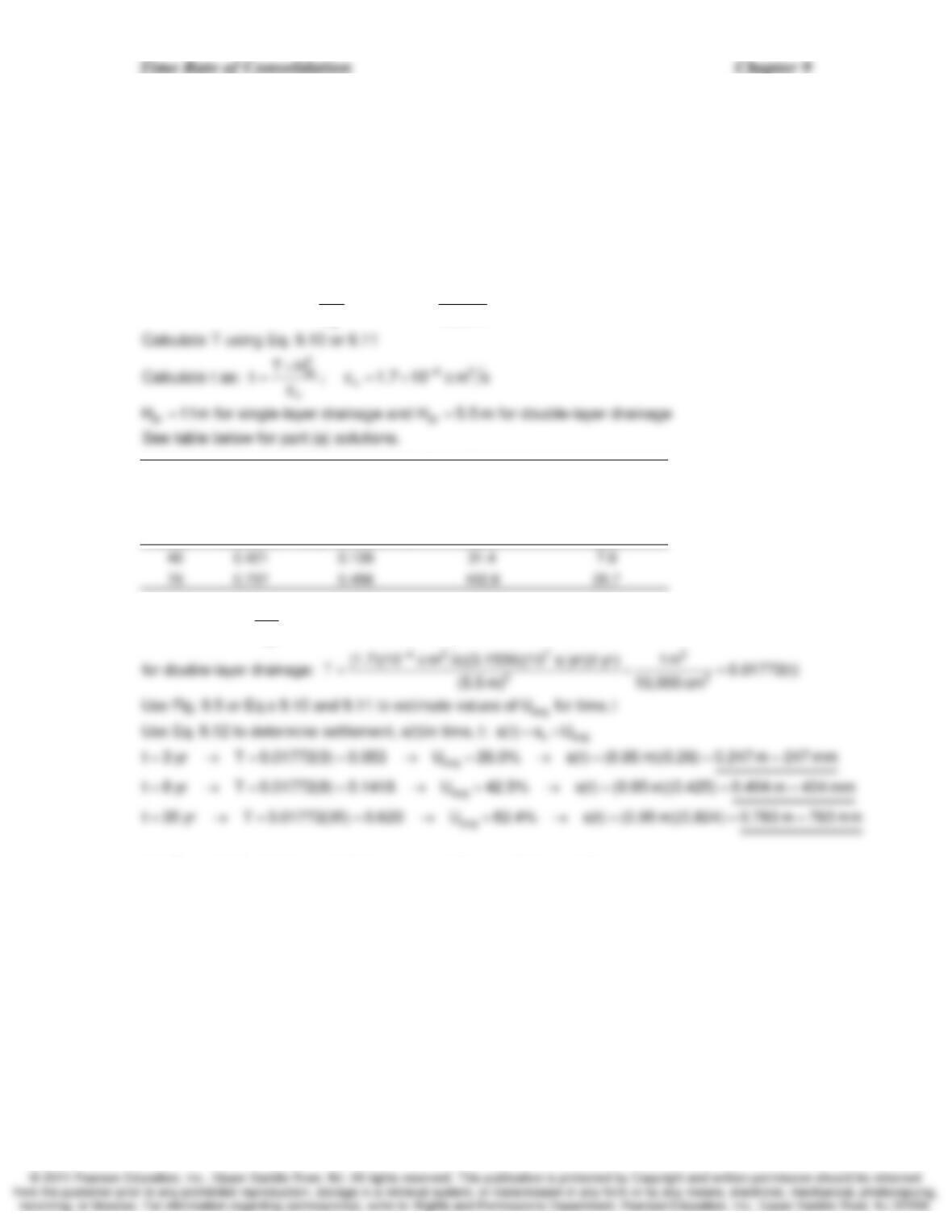
9-8. A deposit of Swedish clay is 11 m thick, on the average, and apparently drained on the
bottom. The coefficient of consolidation for the clay was estimated to be 1.7 x 10⁻⁴ cm2/s from
laboratory tests. A settlement analysis based on consolidation tests predicted an ultimate
consolidation settlement under the applied load in the field to be 0.95 m. (a) How long would it
take for settlements of 40 and 70 cm to occur? (b) How much settlement would you expect to
occur in 3 yr? 8 yr? 35 yr? (c) How long will it take for the ultimate settlement of 0.95 m to occur?
SOLUTION:
avg avg
c
s(t) s(t)
(a) Use Eq. 9.12: U U
s0.95m
=→ =
single drainage H
dr
= 11 m
double drainage
H
dr
= 5.5 m
s(t) U
avg
Ttt
(cm) (decimal) (Eq. 9.10 or 9.11) (yr) (yr)
v
2
dr
ct
(b) Eq. 9.5: T H
=
c
(c) Theoretically, it takes an infinite amount of time to obtain a settlement s .
=
Time Rate of Consolidation Chapter 9
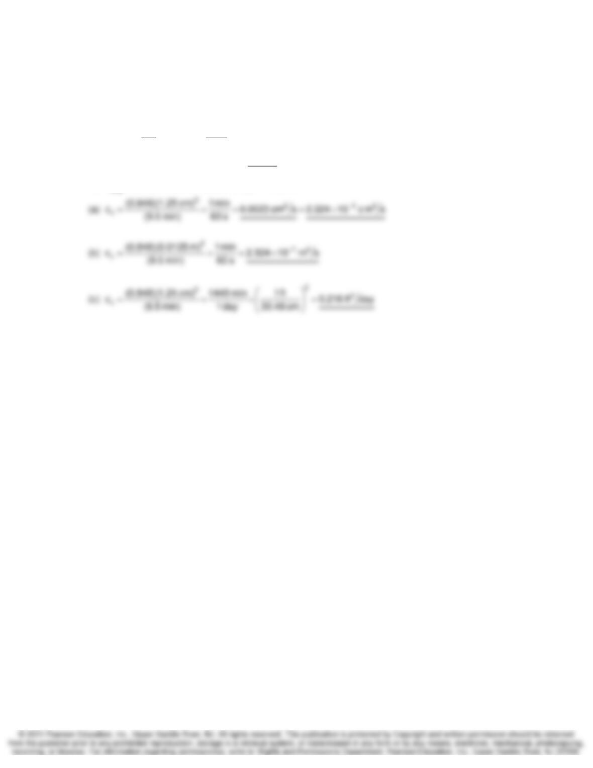
9-9. A conventional laboratory consolidation test on a 25 mm thick sample gave a time for 90%
consolidation equal to 9.5 min. Calculate cv in cm2/s, m2/s, and ft2/d.
SOLUTION:
2
dr
vv
2
dr
dr
avg
TH
ct
Eq. 9.5: T c t
H
2.5 cm
Assume double-layer drainage: H 1.25 cm
2
For U 90%, T 0.848 (Table 9.1), t 9.5 min
=→=
==
== =
Time Rate of Consolidation Chapter 9
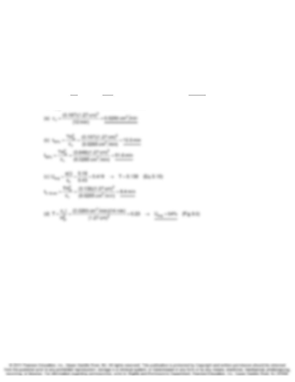
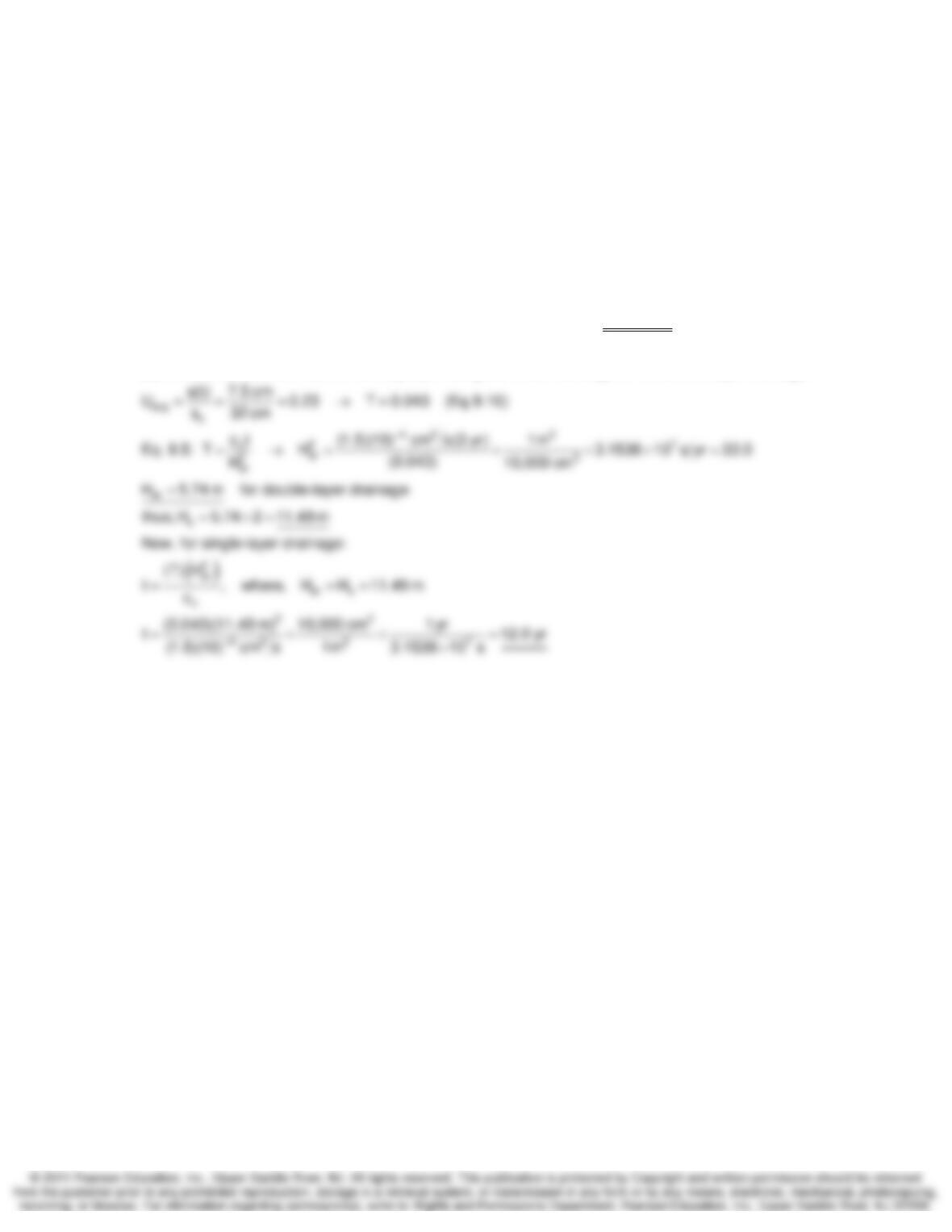
9-10. A doubly drained specimen, 2.54 cm in height, is consolidated in the lab under an applied
stress. The time for 50% overall (or average) consolidation is 12 min. (a) Compute the cv value
for the lab specimen. (b) How long will it take for the specimen to consolidate to an average
consolidation of 50%? (c) If the final consolidation settlement of the specimen is expected to be
0.43 cm, how long will it take for 0.18 cm of settlement to occur? (d) After 14 minutes, what
percent consolidation has occurred at the middle of the specimen?
SOLUTION:
2
dr
vvdr
2
dr
avg
TH
ct 2.54 cm
Eq. 9.5: T c ; For double-layer drainage: H 1.27 cm
t2
H
For U 50%, T 0.197 (Table 9.1), t 12 min
=→= = =
== =
Time Rate of Consolidation Chapter 9
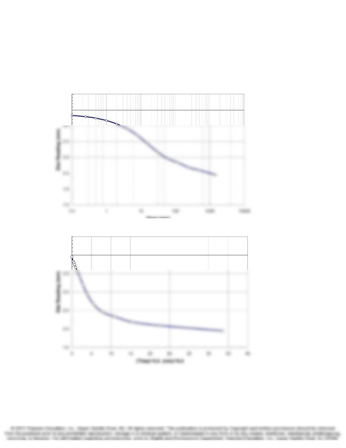
9-11. The settlement analysis for a proposed structure indicates that the underlying clay layer will
settle 7.5 cm in 3 years, and that ultimately the total settlement will be about 32 cm. However, this
analysis is based on the clay layer being doubly drained. It is suspected that there may be no
drainage at the bottom of the layer. Answer the following questions based on single drainage
only, assuming cv = 1.5 x 10⁻⁴ cm2/sec for both single and double drainage. (a) How will the total
settlement change from the double to the single drainage case? (b) How long will it take for 7.5
cm of settlement to occur if there is only single drainage?
SOLUTION:
c
(a) The total settlement for single and double drainage is the same, s 32 cm
(b) Determine the thickness of the clay layer using the initial values given for double-layer drainage.
=
Time Rate of Consolidation Chapter 9
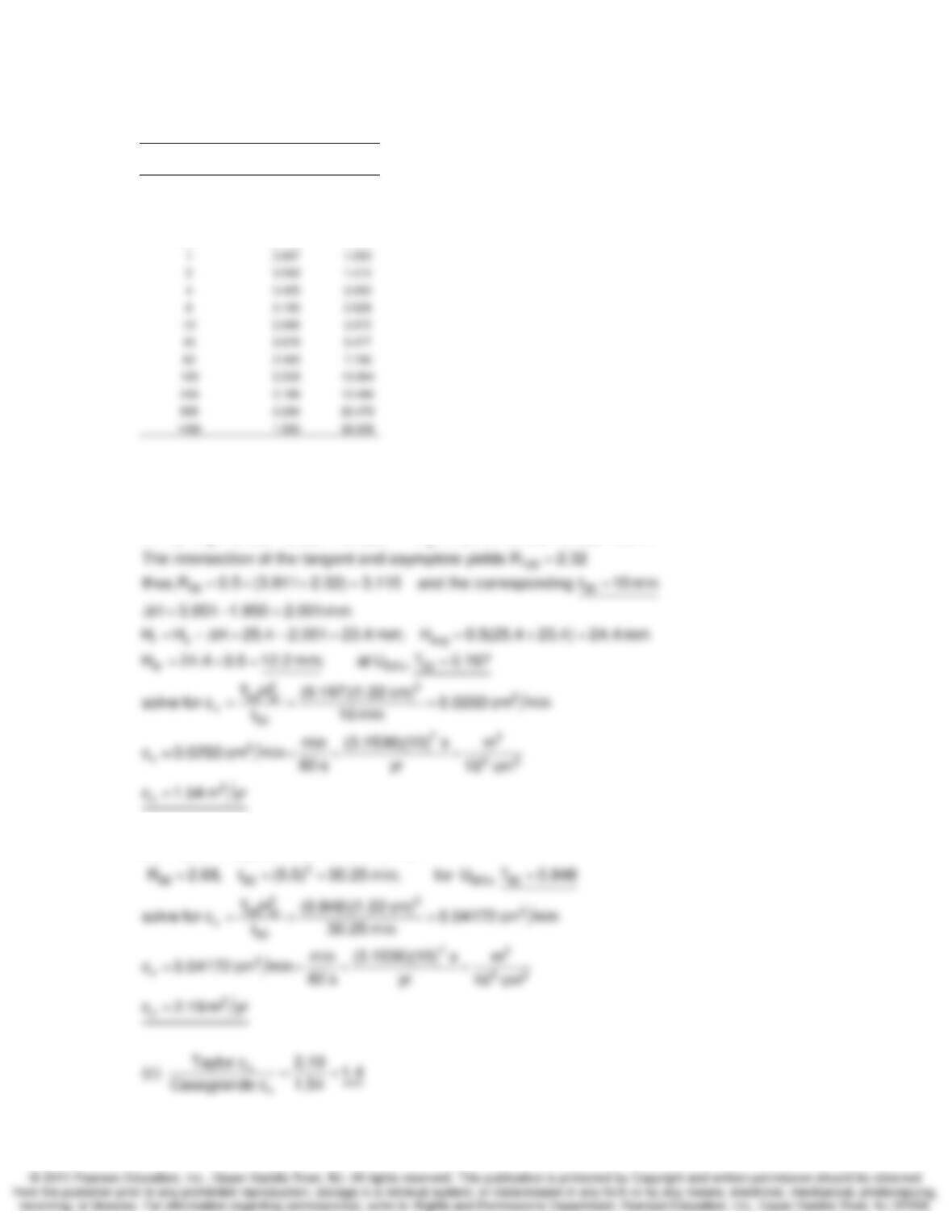
9-13. The time rate of settlement data shown below is for the increment from 20 to 40 kPa from
the test in Fig. 8.5. The initial sample height is 2.54 cm, and there are porous stones on the top
and at the bottom of the sample. Determine cv by: (a) the log time-fitting procedure and (b) the
square root of time procedure. (c) Compare the results of (a) and (b).
SOLUTION:
4.0
4.5
Time (min)
4.0
4.5
Time Rate of Consolidation Chapter 9
9-13 continued.
Elapsed Time, t Dial Reading (t)
0.5
(min) (mm) (min)
1/2
0 3.951 0.000
0.1 3.827 0.316
0.25 3.789 0.500
0.5 3.740 0.707
111122
12 o 1
(a) Casagrande log time-fitting procedure.
select a t choose t 0.25 min (R 3.789), 4t t 1.0 min (R 3.667)
x R R 3.789 3.667 0.122; R R x 3.789 0.122 3.911
→= = ===
=−=−= =+=+=
(b) Taylor ‘ s square root of time method.
Time Rate of Consolidation Chapter 9
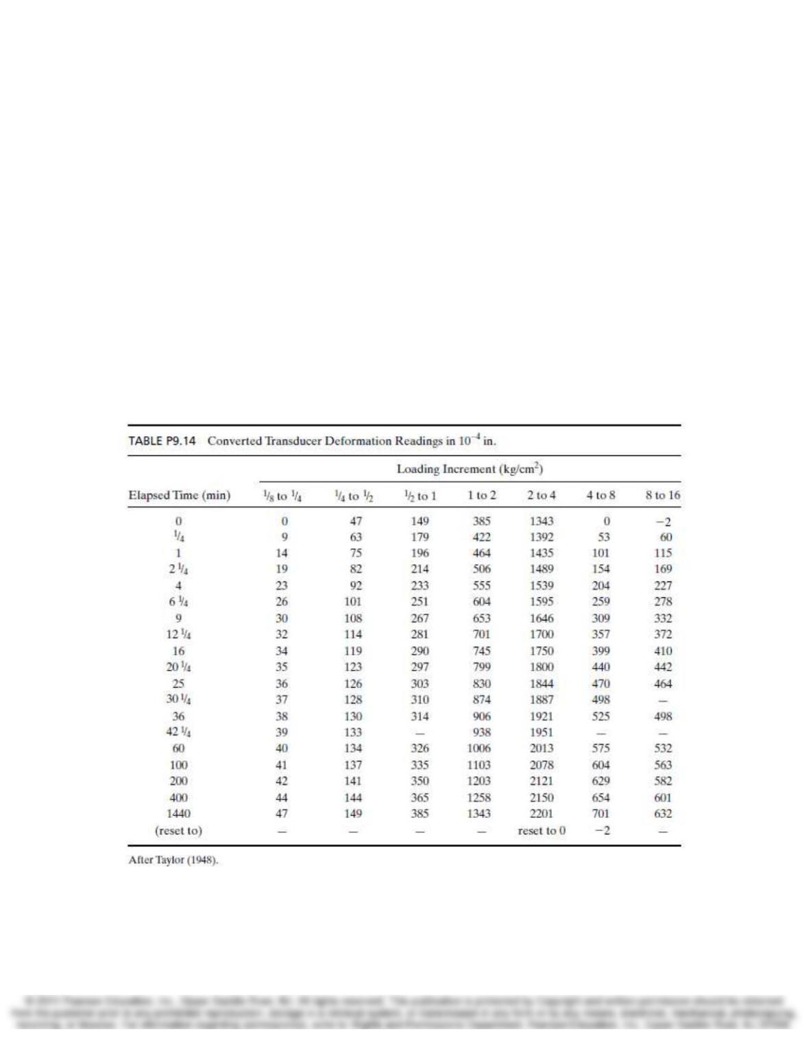
9-14. A consolidation test (Taylor, 1948) was conducted on a sample of soft Chicago silty clay.
The specimen had a dry weight of 343.57 g and a density of solids of 2.65 Mg/m3. The area of the
ring was 93.31 cm2. A displacement transducer was used, which has a precision of one ten-
thousandth of an inch (1 x 10⁻⁴ in), and the incremental stresses applied to the specimen were
recorded in kgf/cm2. Direct measurements of the thickness of the specimen were as follows:
1.254 in when under 1/8 kg/cm2
1.238 in when under 1/2 kg/cm2
1.215 in when under 1 kg/cm2
Deformations to the nearest 10-4 in recorded during the test are listed in Table P9.14. Required:
(a) Use a spreadsheet to plot the e versus log
σ
’ and/or the e versus log
σ
’ curve for this test.
Determine the preconsolidation stress and the appropriate compression index. (b) Use a
spreadsheet to plot dial reading versus (t)1/2 for each increment and determine cv. Plot cv versus
log
σ
’. (c) Same as part (b), only use the Casagrande log time-fitting method. (d) For two
increments, one before and one after the preconsolidation stress, compare the values of cv as
determined by the two fitting procedures.
Time Rate of Consolidation Chapter 9
9.14 continued.
()
−
×
ε= ×
Δ=ε+ = −Δ
=−ε+
4
i
oio
io o
deformation reading 10
Determine strain, : %strain 100
1.254 in
Determine e (e ) at each load:
e(1e);ee e
ee (1e)
(refer to table and plot for solutions)
Transducer
Load Effective Stress Reading Vertical Strain Void Ratio
(kg/cm
2
)(kPa) (10
-4
in) (%) e
0.125 12.263 — — 1.292
Elapsed Transducer
Time Reading
(min) (10
-4
in)
0.00 47
0.25 63
1.00 75
2.25 82
4.00 92
(Time rate readings are for load
increment: ¼ to ½ k
g
/cm2.
)
Time Rate of Consolidation Chapter 9
9.14 continued.
4.0
24.0
0 200 400 600 800 1000 1200 1400 1600
Time (min)
50.0
60.0
70.0
80.0
0.1 1.0 10.0 100.0 1000.0 10000.0
Log time (min)
ε
σ≈
−
==
p
c
From plots:
‘110kPa
30 3
C0.27
100
Time rate readings are for load increment: ¼ to ½ kg/cm2.
Time Rate of Consolidation Chapter 9
9.14 continued.
0.00
5.00
10.00
30.00
10 100 1000 10000
Effective stress (kPa)
1.20
1.30
1.40
Time Rate of Consolidation Chapter 9
9-15. A consolidation test is performed on the specimen with these characteristics:
Height of specimen = 37.60 mm
Area of specimen = 90.1 cm2
Wet weight of specimen = 645.3 g
Dry weight of specimen = 491.2 g
Density of solids = 2.72 Mg/m3
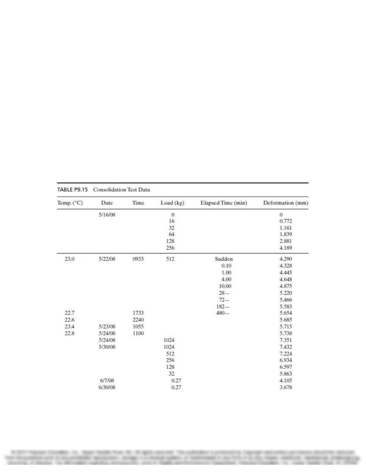
The consolidation data (after A. Casagrande) are summarized in Table P9.15.
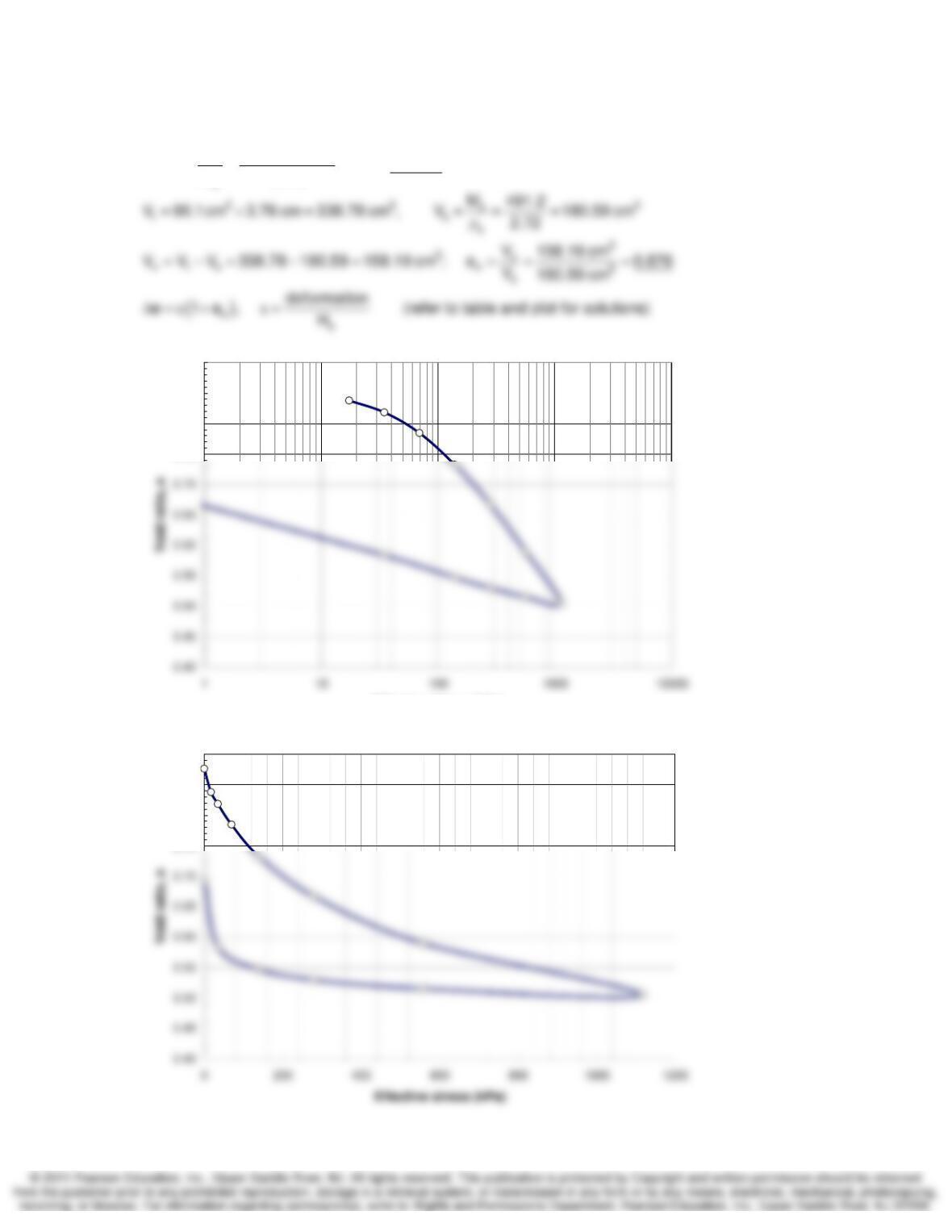
(a) Plot the effective stress versus void ratio curve for both arithmetic and semilogarithmic scales.
(b) Estimate the preconsolidation pressure.
(c) Compute the compression index for virgin consolidation.
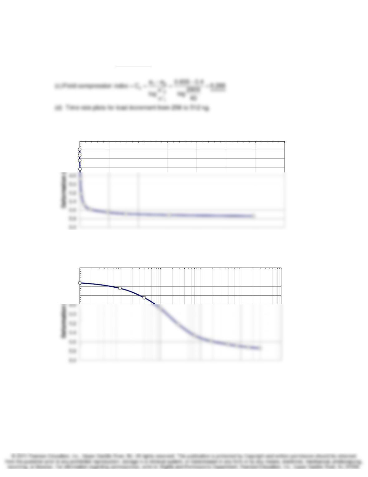
(d) Plot the time curve for the load increment from 256 to 512 kg for both arithmetic and
semilogarithmic scales.
(e) Compute the coefficient of compressibility av, the coefficient of permeability, and the
coefficient of consolidation cv, for the load increment from 256 kg to 512 kg.
Solution continued on next page.
Time Rate of Consolidation Chapter 9
9-15. SOLUTION
wo
s
M645.3 491.2
(a) w 100 31.37% Deter min e e :
M 491.2
−
== ×=
0.75
0.80
0.85
0.90
Effective stress (kPa)
0.75
0.80
0.85
0.90
Time Rate of Consolidation Chapter 9
9-15 continued.
p
(b) From e-log p plot: ‘ 120 kPa
σ≈
4.0
4.2
4.4
4.6
0 500 1000 1500 2000 2500 3000 3500
Time (min)
4.0
4.2
4.4
4.6
0.1 1.0 10.0 100.0 1000.0 10000.0
Log time (min)
Time Rate of Consolidation Chapter 9
9.15 continued.
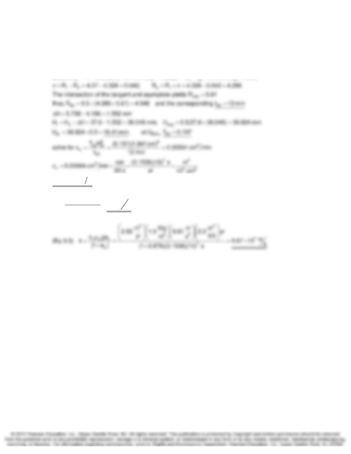
(e) Casagrande log time-fitting procedure.
select a t choose t 0.1min (R 4.328), 4t t 0.4 min (R 4.37)
→== ===
2
v
2
v
c2.92myr
0.667 0.590 m
a 2.0 (for stress increment 278.7 to 557.5 kPa)
kN
557.5 278.7
=
−
==
−