Section 9.2
(–1, 1)
(0, 1)
g(λ) = λ3 + 2λ2 + λ + 1
9.2.14 a For i > 1, dxi
dt =−kixi+xi−1. This means that in the absence of quantity xi−1(t), the quantity xi(t) will
decay exponentially, but the presence of xi−1helps xito grow.
For i= 1, the beginning of the loop, dx1
dt =−k1x1−bxn, so that the presence of xncontributes to the decrease
of x1.
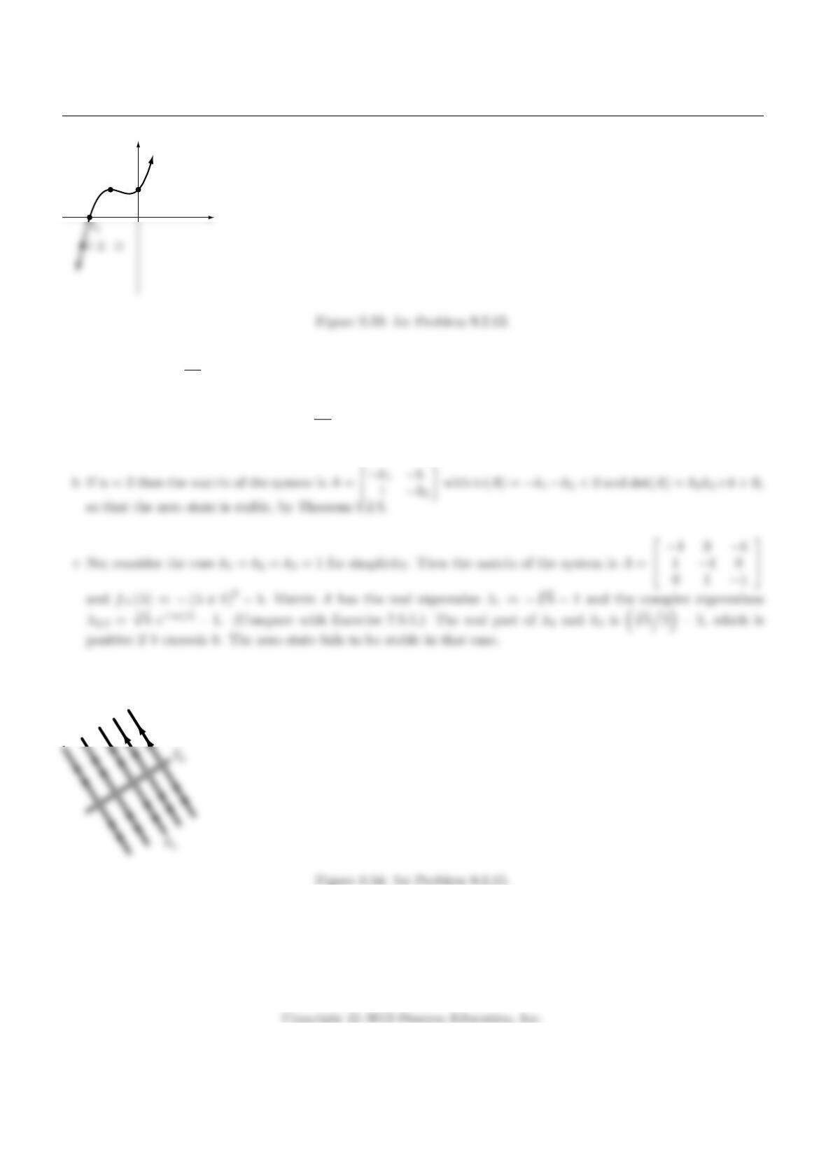
9.2.15 The eigenvalues are λ1= tr(A)>0 and λ2= 0. See Figure 9.34.
9.2.16 If A=0 1
a b then tr(A) = band det(A) = −a. By Theorem 9.2.5, the zero state is stable if aand bare
both negative.
427
Chapter 9
9.2.17 If A=−1k
k−1then tr(A) = −2 and det(A) = 1 −k2. By Theorem 9.2.5, the zero state is stable if
det(A) = 1 −k2>0, that is, if |k|<1.
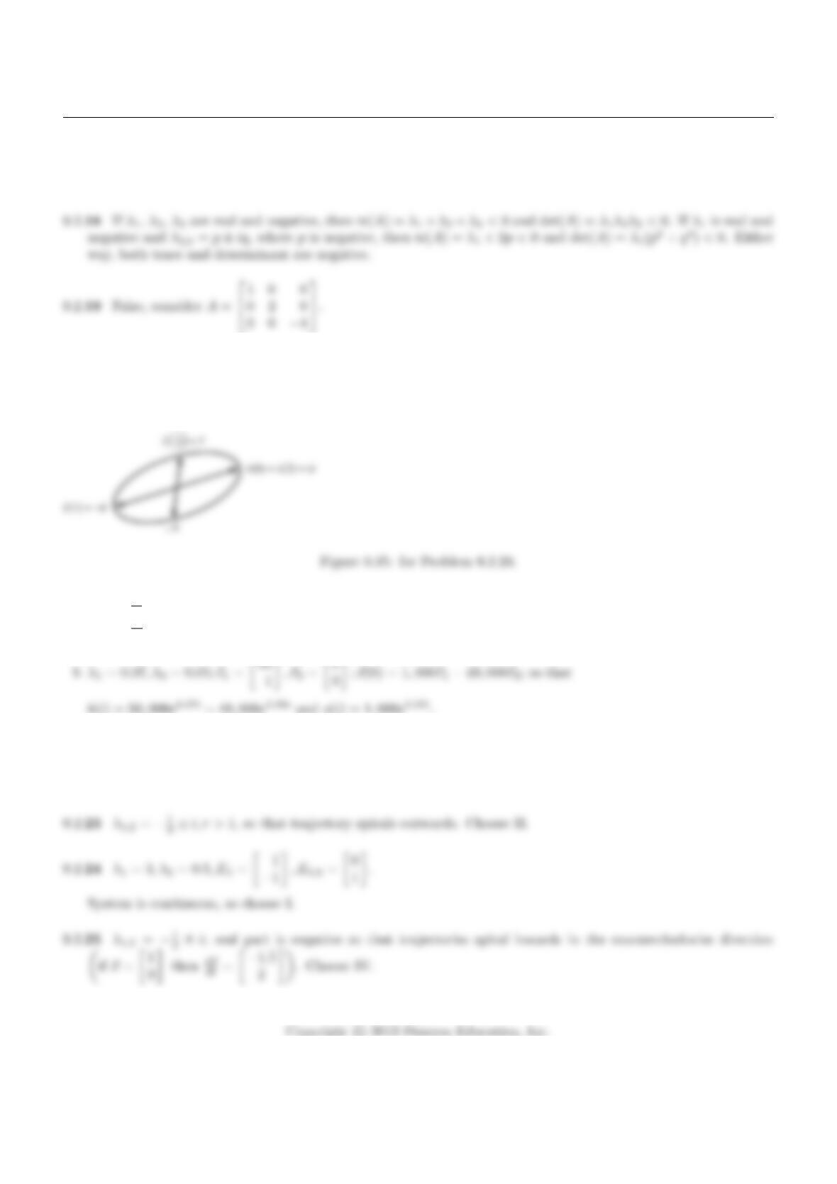
9.2.20 Use Theorem 9.2.6, with p= 0, q =π;a= 1, b = 0.
~x(t) = [ ~w ~v ]cos(πt)−sin(πt)
sin(πt) cos(πt)1
0= (cos(πt)) ~w + (sin(πt))~v. See Figure 9.35.
9.2.21 adb
dt = 0.05b+s
ds
dt = 0.07sand b(0)
s(0) =1,000
1,000
9.2.22 λ1= 3, λ2= 0.5; E3= span 1
−1, E0.5= span 0
1
System is discrete so choose VII.
428
Section 9.2
9.2.26 λ1= 1, λ2=−2; E1= span 0
1, E−2= span 1
−1.
System is continuous so choose V.
9.2.28 λ1,2=±6i, E6i= span 2
0+i0
3, so that
~x(t) = 0 2
3 0 cos(6t)−sin(6t)
sin(6t) cos(6t)a
b=2 sin(6t) 2 cos(6t)
3 cos(6t)−3 sin(6t)a
b.
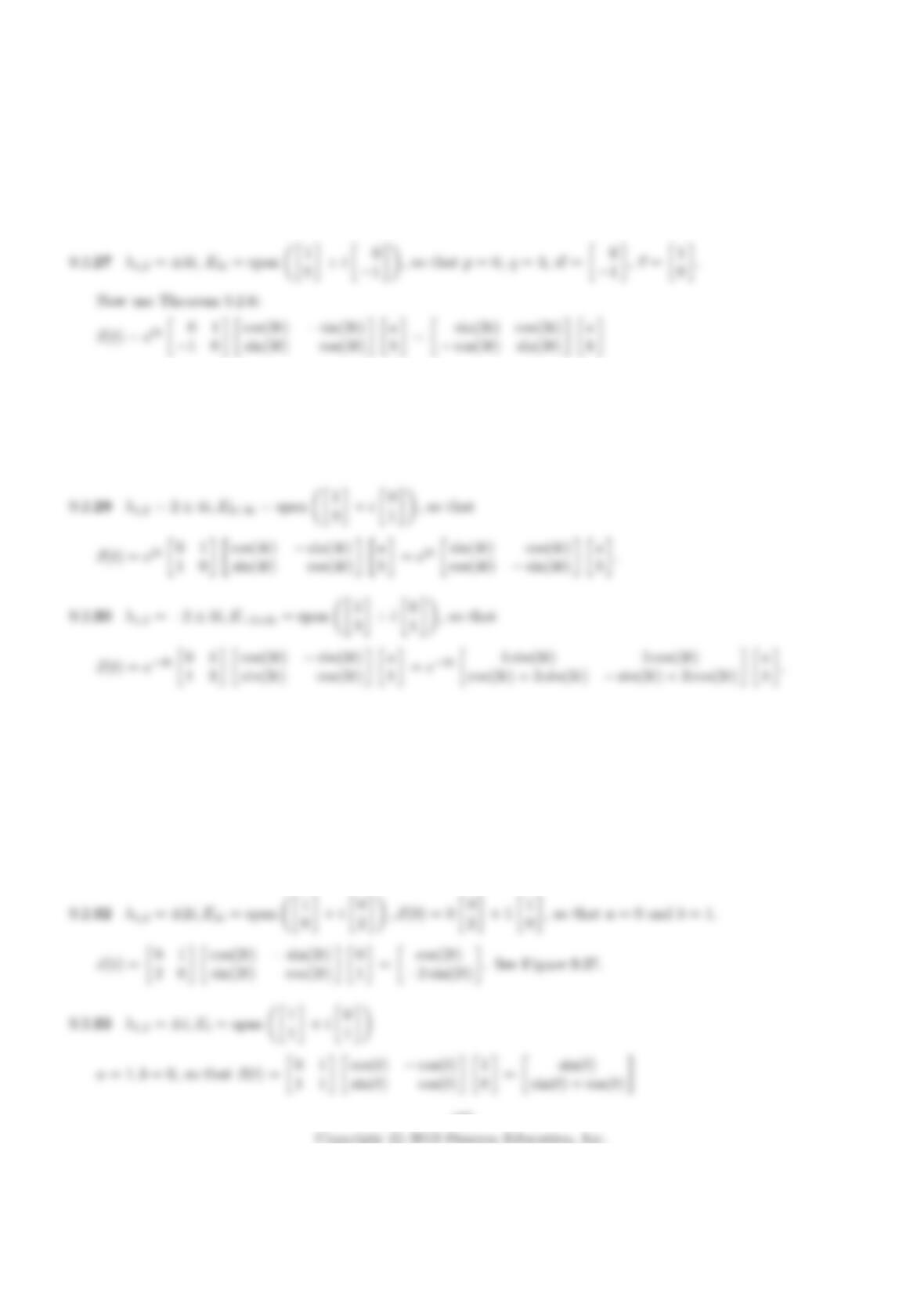
9.2.31 λ1,2=−1±2i, E−1+2i= span 1
0+i0
−1, so that p=−1, q = 2, ~w =0
−1,
~v =1
0. Now 1
−1=~x(0) = ~w +~v, so that a= 1 and b= 1.
Then ~x(t) = e−t0 1
−1 0 cos(2t)−sin(2t)
sin(2t) cos(2t)1
1=e−tsin(2t) + cos(2t)
sin(2t)−cos(2t).
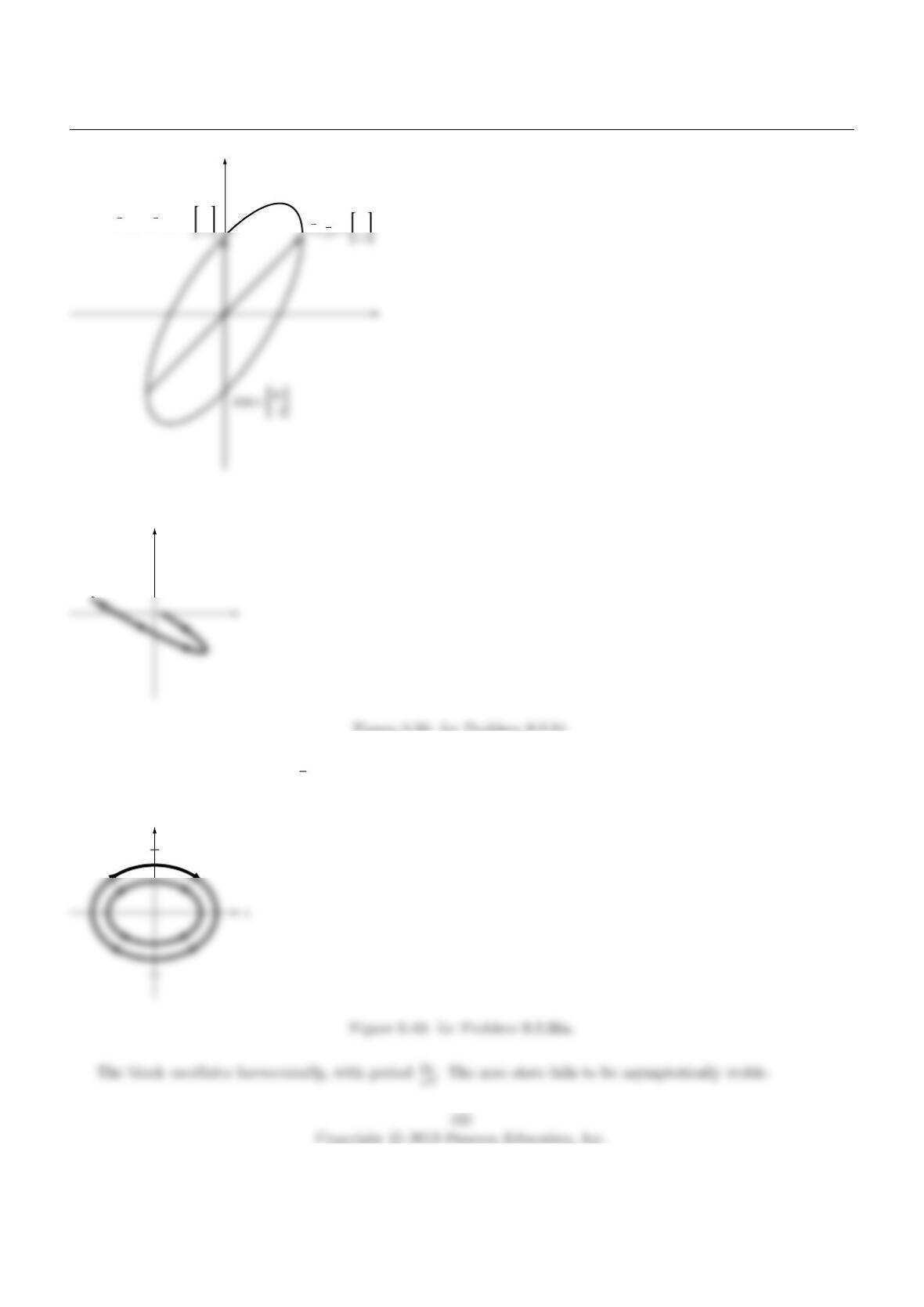
See Figure 9.36.
429
Chapter 9
1
1
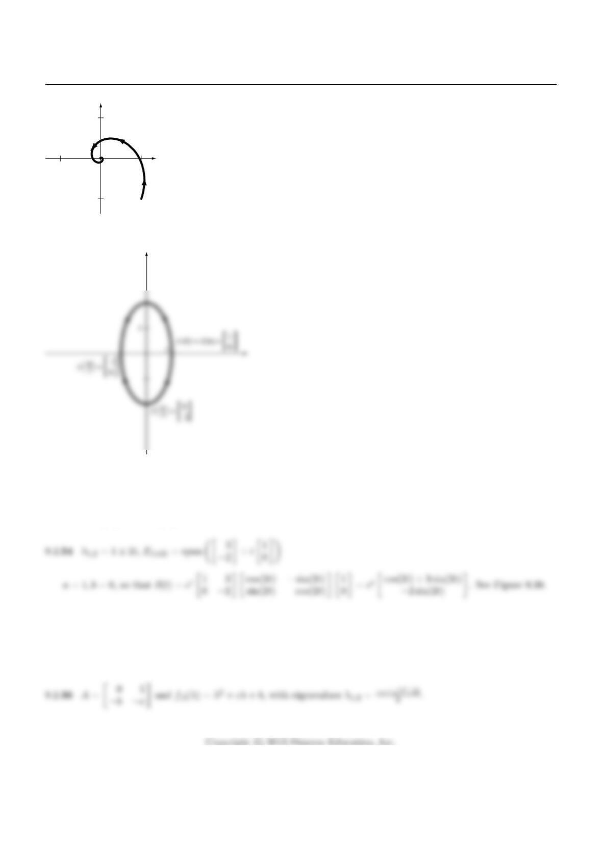
Figure 9.36: for Problem 9.2.31.
Figure 9.37: for Problem 9.2.32.
= cos(t)0
1+ sin(t)1
1. See Figure 9.38.
9.2.35 If z=f+ig and w=p+iq then zw = (f p −gq) + i(f q +gp), so that (zw)′= (f′p+fp′−g′q−gq′) +
i(f′q+fq′+g′p+gp′).
Also z′w= (f′+ig′)(p+iq) = (f′p−g′q) + i(f′q+g′p) and zw′= (f+ig)(p′+iq′) = (fp′−gq′) + i(gp′+fq′).
We can see that (zw)′=z′w+zw′, as claimed.
430
Section 9.2
1
=
x
π
0
=
x (0) = x(2π)
Figure 9.38: for Problem 9.2.33.
Figure 9.39: for Problem 9.2.34.
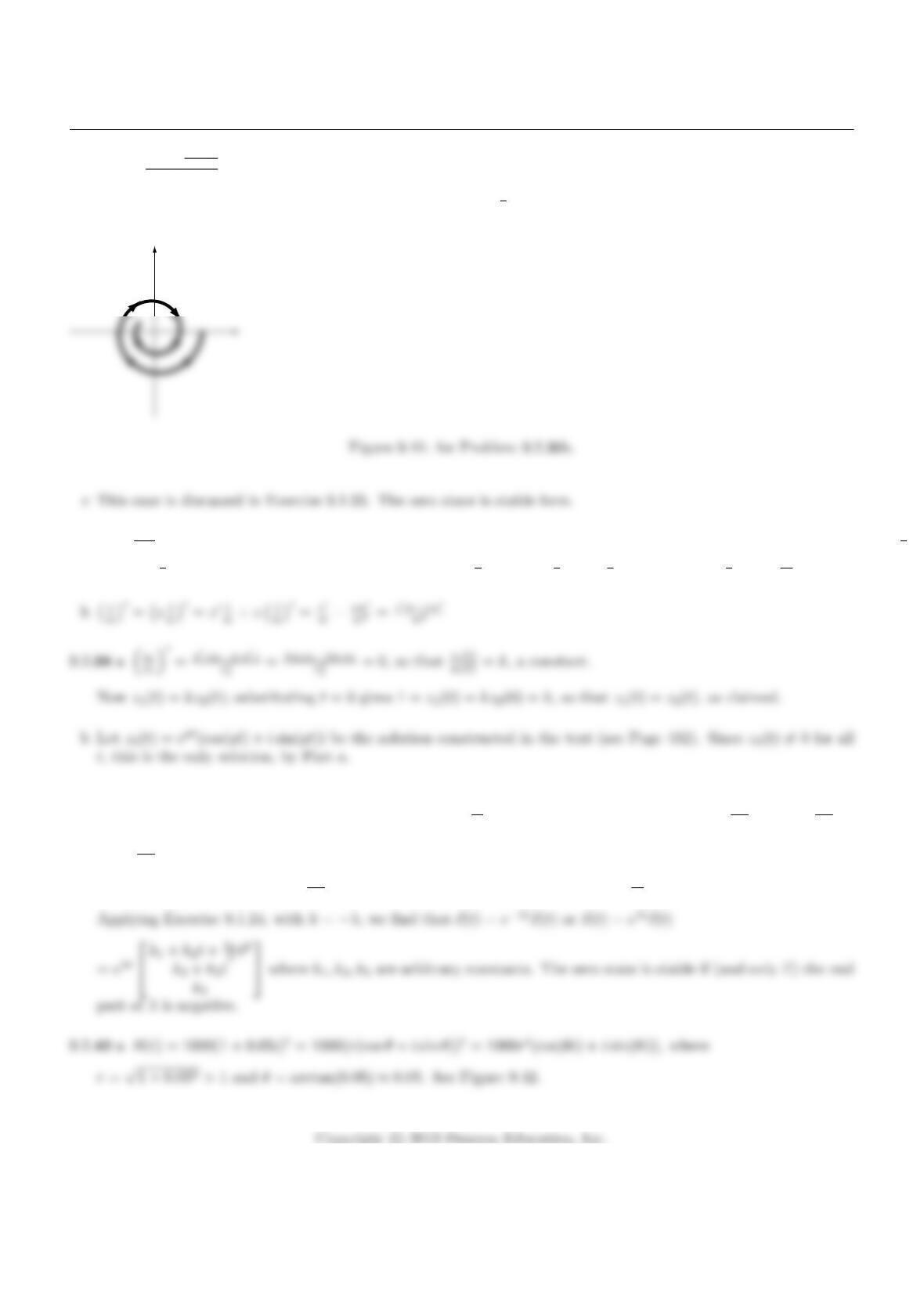
9.2.36 a If c= 0 then λ1,2=±i√b. The trajectories are ellipses. See Figure 9.40.
v
Chapter 9
bλ1,2=−c±i√4b−c2
2
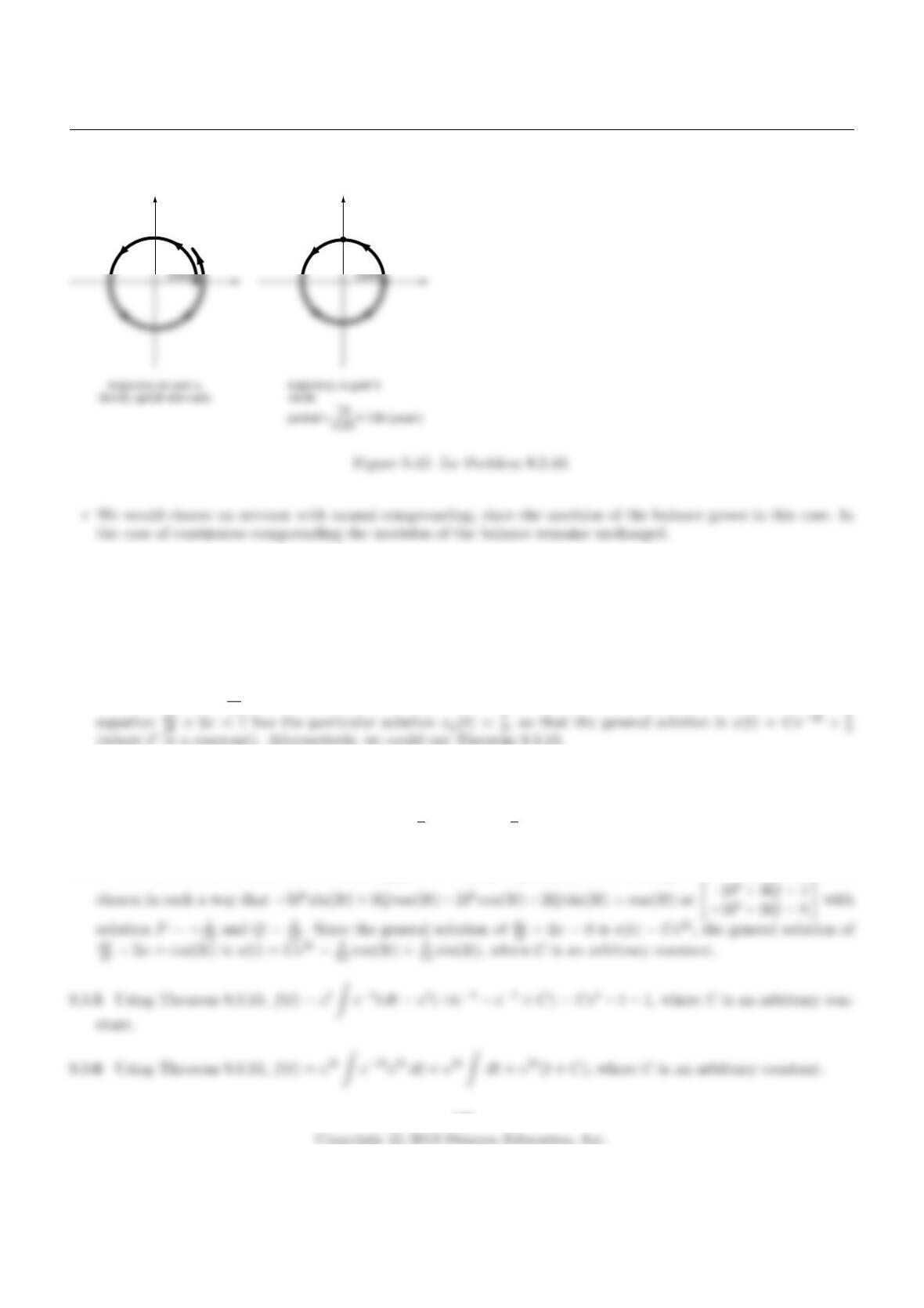
The trajectories spiral inwards, since Re(λ1) = Re(λ2) = −c
2<0. This is the case of a damped oscillation. The
zero state is asymptotically stable. See Figure 9.41.
9.2.37 a1
z(t)is differentiable when z(t)6= 0, since both the real and the imaginary parts are differentiable if z=p+iq then 1
z=
To find 1
z′, apply the product rule to the equation z1
z= 1: z′1
z+z1
z′= 0, so that 1
z′=−z′
z2.
9.2.39 Let A=
λ1 0
0λ1
0 0 λ
. We first solve the system d~c
dt = (A−λI3)~c =
0 1 0
0 0 1
0 0 0
~c, or dc1
dt =c2(t),dc2
dt =
c3(t),dc3
dt = 0.
c3(t) = k3, a constant, so that dc2
dt =k3and c2(t) = k3t+k2. Likewise c1(t) = k3
2t2+k2t+k1.
432
Section 9.3
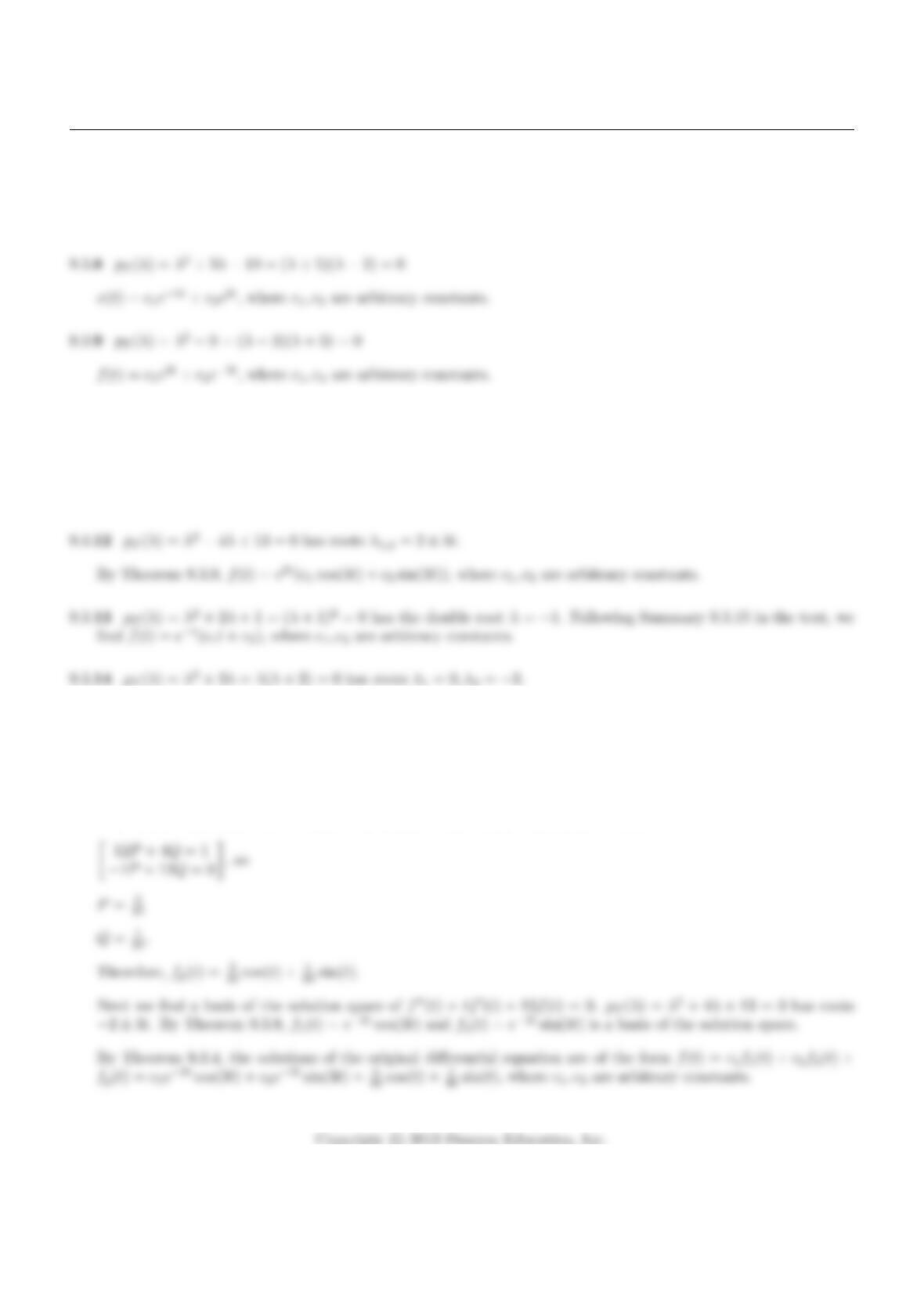
bB(t) = 1000e0.05i= 1000(cos(0.05t) + isin(0.05t)). See Figure 9.42.
1000
Section 9.3
9.3.1The characteristic polynomial of this differential equation is λ−5, so that λ1= 5. By Theorem 9.3.8 the
general solution is f(t) = Ce5t, where Cis an arbitrary constant.
9.3.2The solutions of dx
dt +3x= 0 are of the form x(t) = Ce−3t, where Cis an arbitrary constant, and the differential
9.3.3Use Theorem 9.3.13, where a=−2 and g(t) = e3t:
f(t) = e−2tZe2te3tdt =e−2tZe5tdt =e−2t1
5e5t+C=1
5e3t+Ce−2t, where Cis a constant.
9.3.4We can look for a sinusoidal solution xp(t) = Pcos(3t) + Qsin(3t), as in Example 7. Pand Qneed to be
433
Chapter 9
9.3.7By Definition 9.3.6, pT(λ) = λ2+λ−12 = (λ+ 4)(λ−3).
Since pT(λ) has distinct roots λ1=−4 and λ2= 3, the solutions of the differential equation are of the form
f(t) = c1e−4t+c2e3t, where c1and c2are arbitrary constants (by Theorem 9.3.8).
9.3.10 pT(λ) = λ2+ 1 = 0 has roots λ1,2=±i. By Theorem 9.3.9, f(t) = c1cos(t) + c2sin(t), where c1, c2are
arbitrary constants.
9.3.11 pT(λ) = λ2−2λ+ 2 = 0 has roots λ1,2= 1 ±i. By Theorem 9.3.9, x(t) = et(c1cos(t) + c2sin(t)), where
c1, c2are arbitrary constants.
9.3.15 By integrating twice we find f(t) = c1+c2t, where c1, c2are arbitrary constants.
9.3.16 By Theorem 9.3.10, the differential equation has a particular solution of the form fp(t) = Pcos(t) + Qsin(t).
Plugging fpinto the equation we find
(−Pcos(t)−Qsin(t)) + 4(−Psin(t) + Qcos(t)) + 13(Pcos(t) + Qsin(t)) = cos(t) or
434
Section 9.3
9.3.17 By Theorem 9.3.10, the differential equation has a particular solution of the form fp(t) = Pcos(t) + Qsin(t).
9.3.18 We follow the approach outlined in Exercises 16 and 17.
9.3.19 We follow the approach outlined in Exercise 17.
•Particular solution xp(t) = cos(t)
9.3.20 pT(λ) = λ3−3λ2+ 2λ=λ(λ−1)(λ−2) = 0 has roots λ1= 0, λ2= 1, λ3= 2.
By Theorem 9.3.8, the general solution is f(t) = c1+c2et+c3e2t, where c1, c2, c3are arbitrary constants.
9.3.23 General solution f(t) = Ce5t
Plug in: 3 = f(0) = Ce0=C, so that f(t) = 3e5t.
9.3.25 General solution f(t) = Ce−2t
Plug in: 1 = f(1) = Ce−2, so that C=e2and f(t) = e2e−2t=e2−2t.
435
Chapter 9
9.3.26 General solution f(t) = c1e3t+c2e−3t(see Exercise 9), with f′(t) = 3c1e3t−3c2e−3t
Plug in: 0 = f(0) = c1+c2and 1 = f′(0) = 3c1−3c2, so that c1=1
6, c2=−1
6, and f(t) = 1
6e3t−1
6e−3t.
9.3.29 General solution f(t) = c1cos(2t) + c2sin(2t) + 1
3sin(t), so that f′(t) = −2c1sin(2t) + 2c2cos(2t) + 1
3cos(t)
(use the approach outlined in Exercise 17)
Plug in: 0 = f(0) = c1and 0 = f′(0) = 2c2+1
3, so that c1= 0, c2=−1
6, and f(t) = −1
6sin(2t) + 1
3sin(t).
9.3.30 akis a positive constant that depends on the rate of cooling of the coffee (it varies with the material of the
cup, for example).
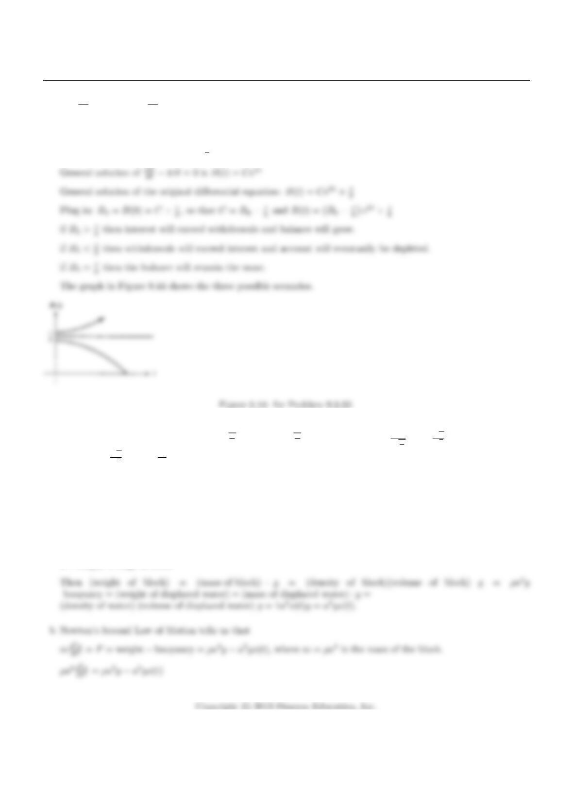
9.3.31 dv
dt +k
mv=g
constant particular solution: vp=mg
k
Section 9.3
9.3.32 dB
dt =kB −ror dB
dt −kB =−r
↑
interest ↑
withdrawals
constant particular solution Bp=r
k
9.3.33 By Theorem 9.3.9, x(t) = c1cos pg
Lt+c2sin pg
Lt, with period P=2π
√g
L
= 2π√L
√g. It is required that
2 = P= 2π√L
√gor L=g
π2≈0.994 (meters).
9.3.34 a We will take downward forces as positive.
Let g= acceleration due to gravity,
ρ= density of block
a= length of edge of block
437
Chapter 9
d2x
dt2=g−g
ρa x(t)
d2x
dt2+g
ρa x=g
constant solution xp=ρa
9.3.35 apT(λ) = λ2+ 3λ+ 2 = (λ+ 1)(λ+ 2) = 0 with roots λ1=−1 and λ2=−2, so x(t) = c1e−t+c2e−2t.
bx′(t) = −c1e−t−2c2e−2t
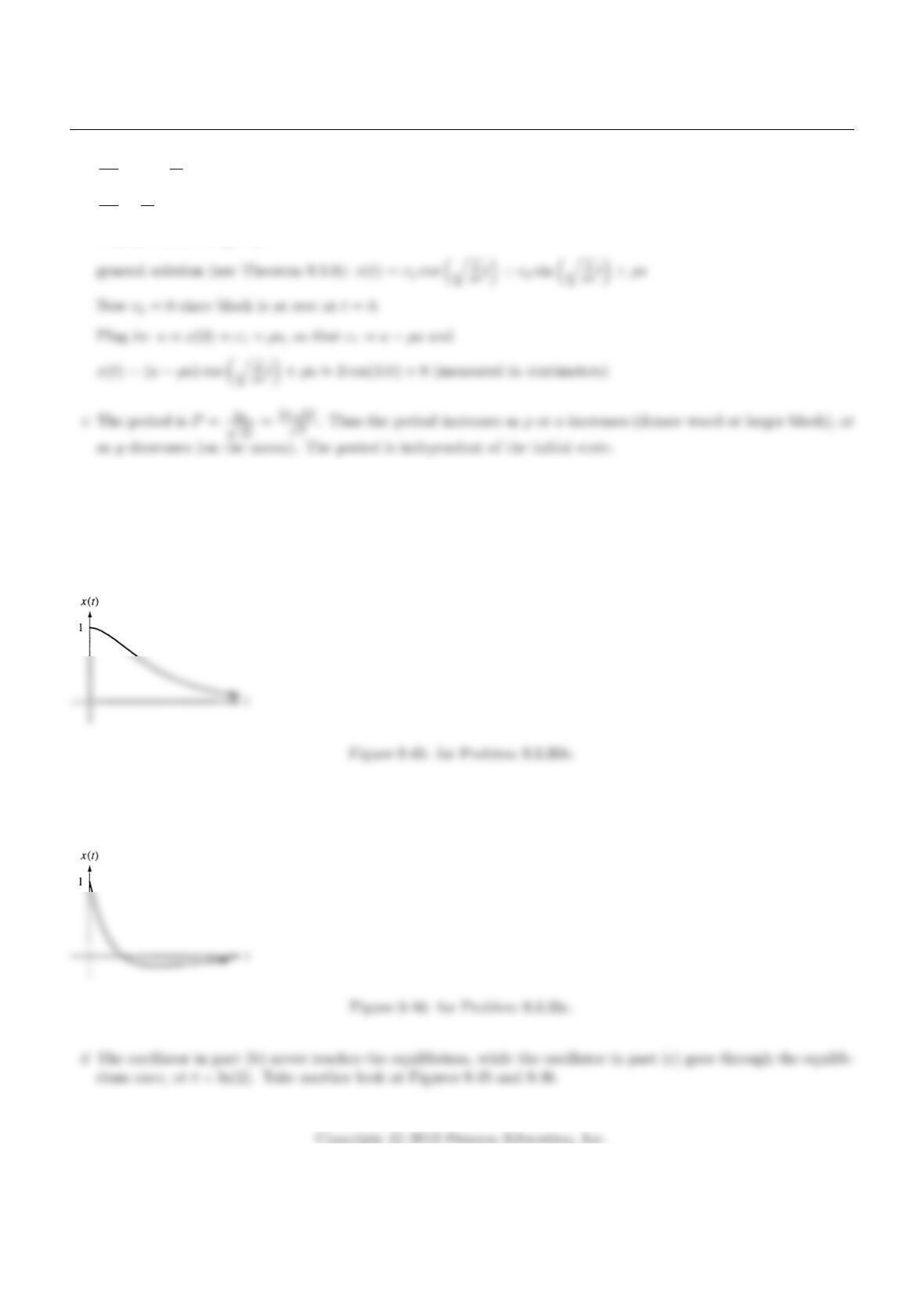
Plug in: 1 = x(0) = c1+c2and 0 = x′(0) = −c1−2c2, so that c1= 2, c2=−1 and x(t) = 2e−t−e−2t. See Figure
9.45.
c Plug in: 1 = x(0) = c1+c2and −3 = x′(0) = −c1−2c2, so that c1=−1, c2= 2, and x(t) = −e−t+ 2e−2t. See
Figure 9.46.
438
Section 9.3
9.3.36 fT(λ) = λ2+ 2λ+ 101 = 0 has roots λ1,2=−1±20i.
By Theorem 9.3.9, x(t) = e−t(c1cos(20t) + c2sin(20t)).
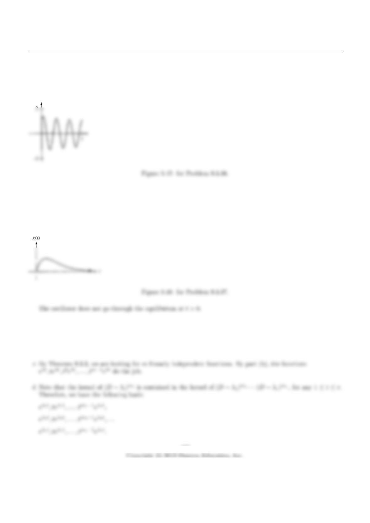
Any nonzero solution goes through the equilibrium infinitely many times. See Figure 9.47.
9.3.37 fT(λ) = λ2+ 6λ+ 9 = (λ+ 3)2has roots λ1,2=−3.
Following the method of Example 10, we find the general solution x(t) = e−3t(c1+c2t) with x′(t) = e−3t(c2−
3c1−3c2t).
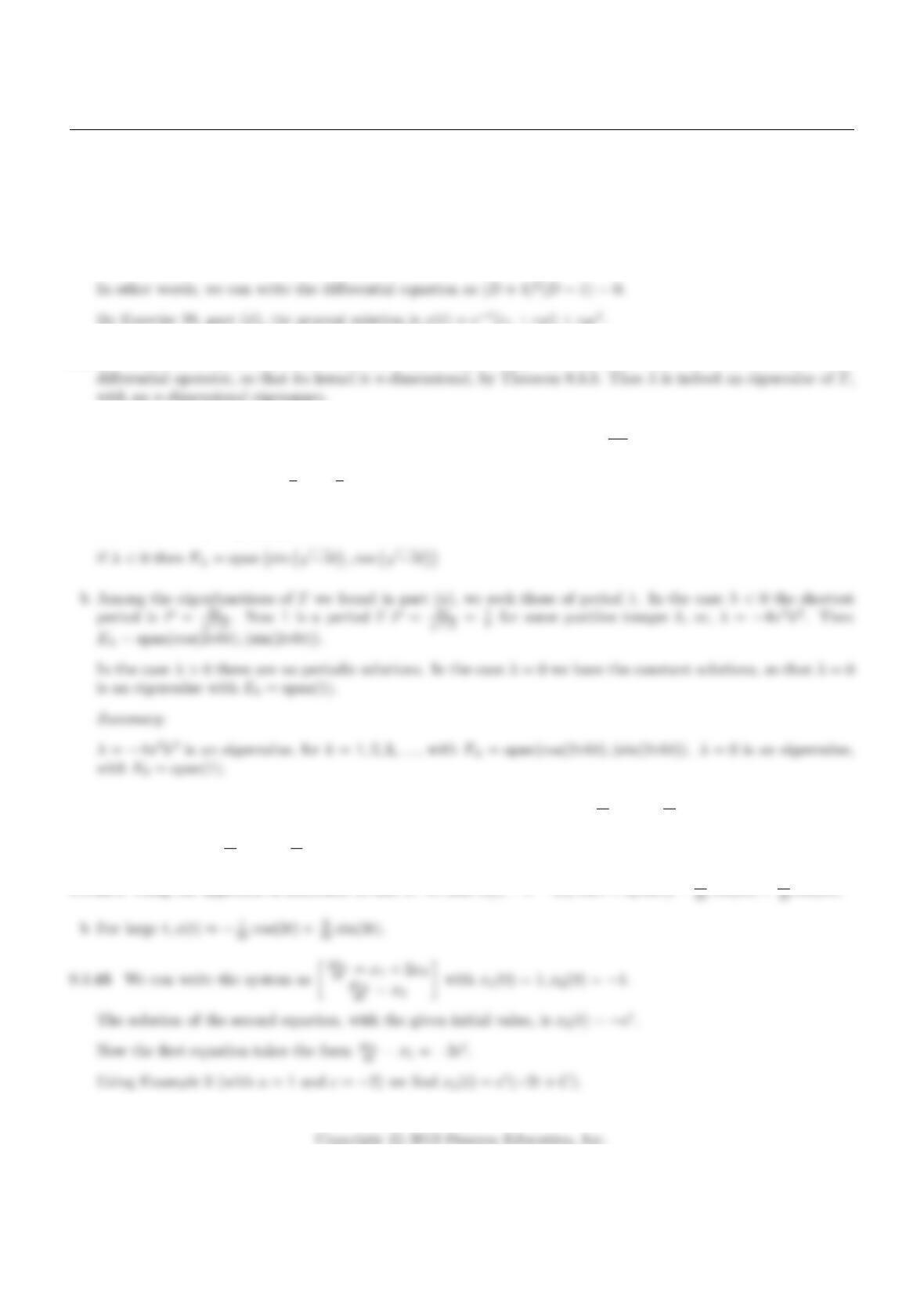
Plug in: 0 = x(0) = c1, and 1 = x′(0) = c2−3c1, so that c1= 0, c2= 1, and x(t) = te−3t. See Figure 9.48.
9.3.38 a (D−λ)(p(t)eλt) = [p(t)eλt]′−λp(t)eλt =p′(t)eλt +λp(t)eλt −λp(t)eλt =p′(t)eλt, as claimed.
b Applying the result from part (a) mtimes we find (D−λ)m(p(t)eλt) = p(m)(t)eλt = 0, since p(m)(t) = 0 for a
polynomial of degree less than m.
439
Chapter 9
9.3.39 fT(λ) = λ3+ 3λ2+ 3λ+ 1 = (λ+ 1)3= 0 has roots λ1,2,3=−1. In other words, we can write the differential
equation as (D+ 1)3f= 0.
By Exercise 38, part (c), the general solution is f(t) = e−t(c1+c2t+c3t2).
9.3.40 fT(λ) = λ3+λ2−λ−1 = (λ+ 1)2(λ−1) = 0 has roots λ1,2=−1, λ3= 1.
9.3.41 We are looking for functions xsuch that T(x) = λx, or T(x)−λx = 0. Now T(x)−λx is an nth-order linear
9.3.42 a We need to solve the second-order differential equation T x =D2x=d2x
dt2=λx. This differential equation
has a two-dimensional solution space Eλfor any λ, so that all λare eigenvalues of T.
if λ > 0 then Eλ= span e√λt, e−√λt
if λ= 0 then Eλ= span(1, t)
9.3.43 a Using the approach of Exercise 17, we find x(t) = c1e−2t+c2e−3t+1
10 cos t+1
10 sin t.
b For large t, x(t)≈1
10 cos t+1
10 sin t.
9.3.44 a Using the approach of Exercises 16 and 17 we find x(t) = e−2t(c1cos t+c2sin t)−1
440
Section 9.3
9.3.46 We can write the system as
dx1
dt = 2x1+ 3x2+x3
dx2
dt =x2+ 2x3
dx3
dt =x3
with x1(0) = 2, x2(0) = 1, x3(0) = −1 .
We solve for x2and x3as in Exercise 45:
x2(t) = et(1 −2t)
9.3.47 a We start with a preliminary remark that will be useful below: If f(t) = p(t)eλt, where p(t) is a polynomial,
then f(t) has an antiderivative of the form q(t)eλt, where q(t) is another polynomial. We leave this remark as a
calculus exercise.
The function xn(t) satisfies the differential equation dxn
dt =annxn, so that xn=Ceann t, which is of the de-
sired form.
b It is shown in introductory calculus classes that lim
t→∞(tmeλt) = 0 if and only if λis negative (here mis a fixed
positive integer). In light of part (a), this proves the claim.
441
Chapter 9
9.3.48 a By Exercise 47, the system d~u
dt =B~u has a unique solution ~u(t). Then the system d~x
dt =A~x has the unique
solution ~x(t) = S~u(t).
442