Hence, for any x-location
=
A
QQ
or
()
δ
=−
*
A
Uy U y
or
where
m
x∼
0.03
0.035
0.04
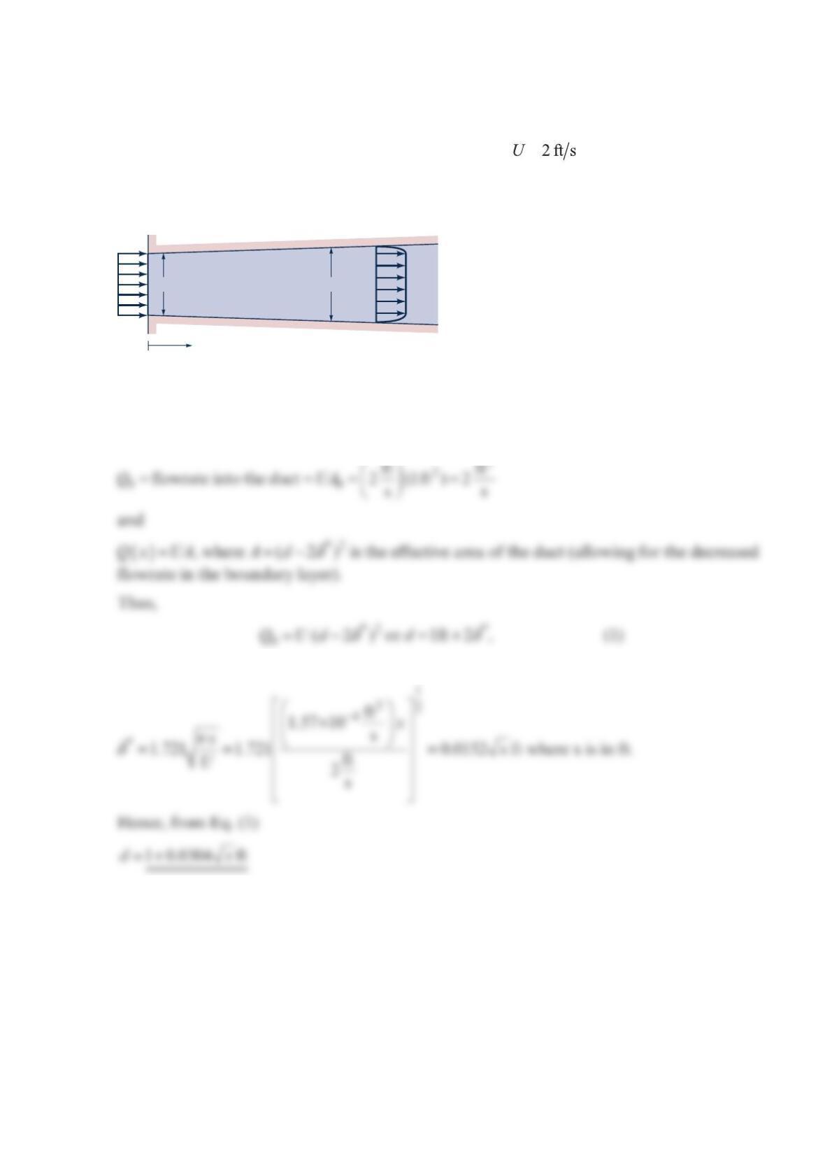
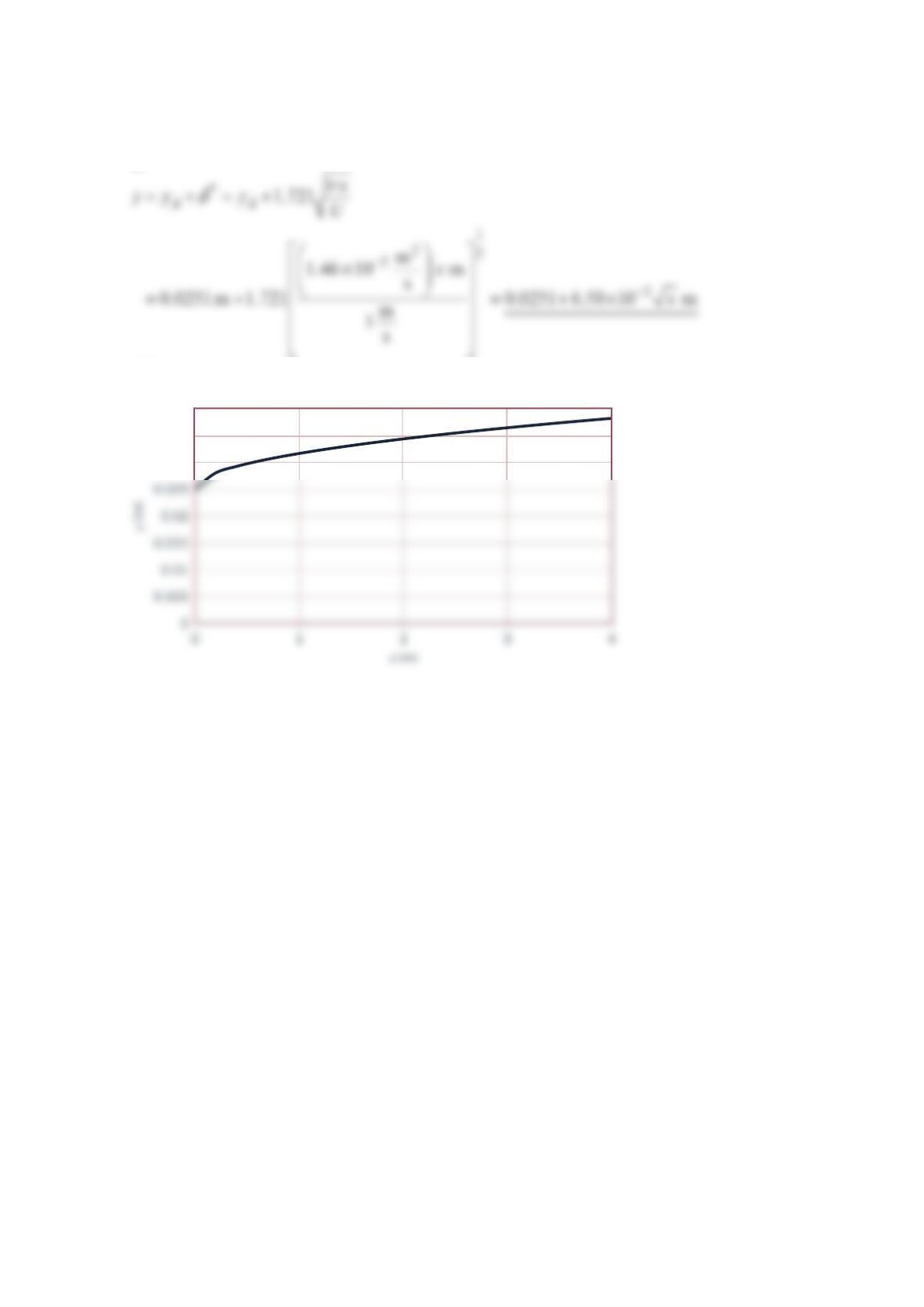
Problem 9.19
Air enters a square duct through a
1
-ft opening as shown in the figure below. Because the
boundary layer displacement thickness increases in the direction of flow, it is necessary to
increase the cross-sectional size of the duct if a constant = velocity is to be
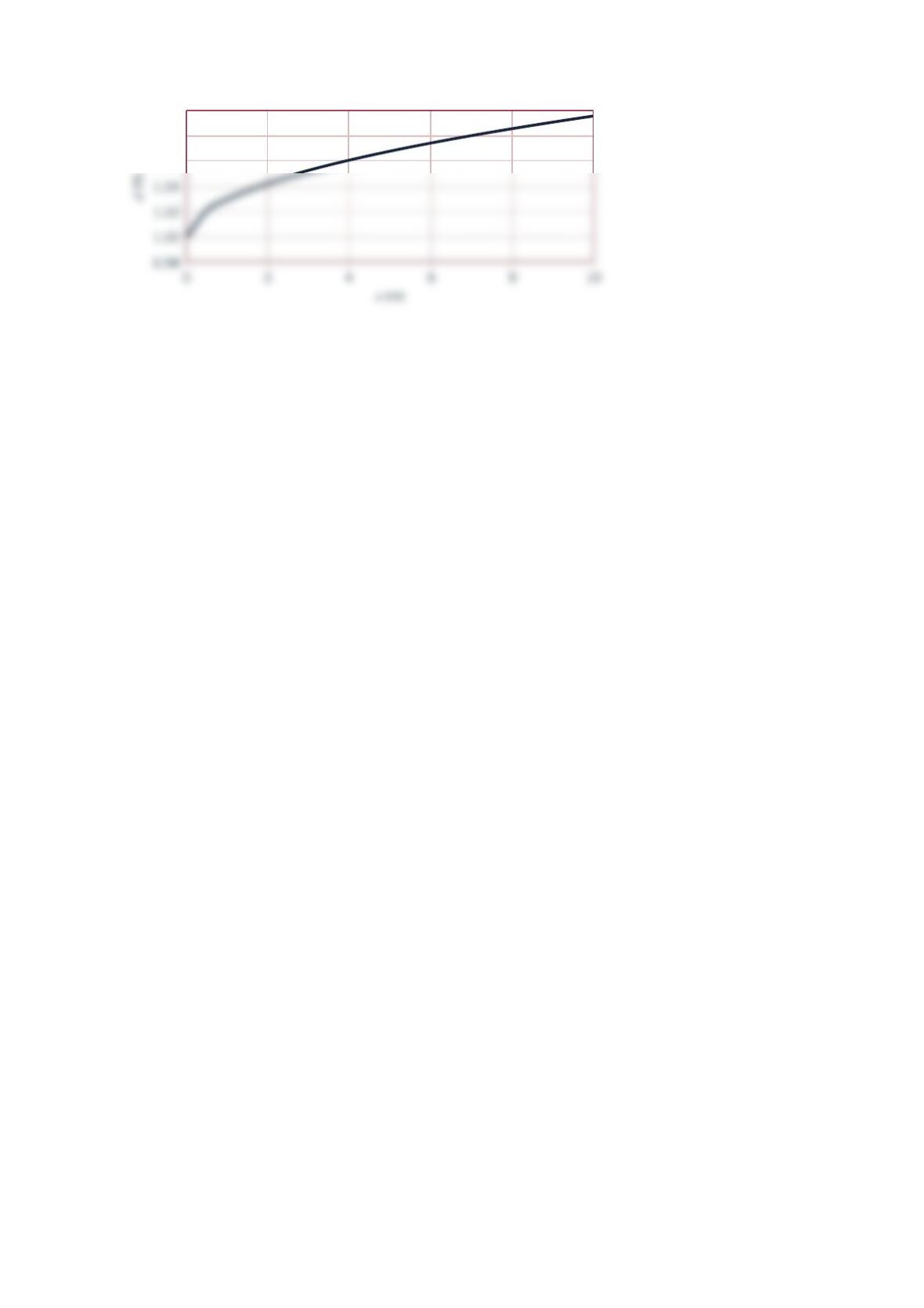
maintained outside the boundary layer. Plot a graph of the duct size, d, as a function of x
for ≤≤010ftx if U is to remain constant. Assume laminar flow.
Solution 9.19
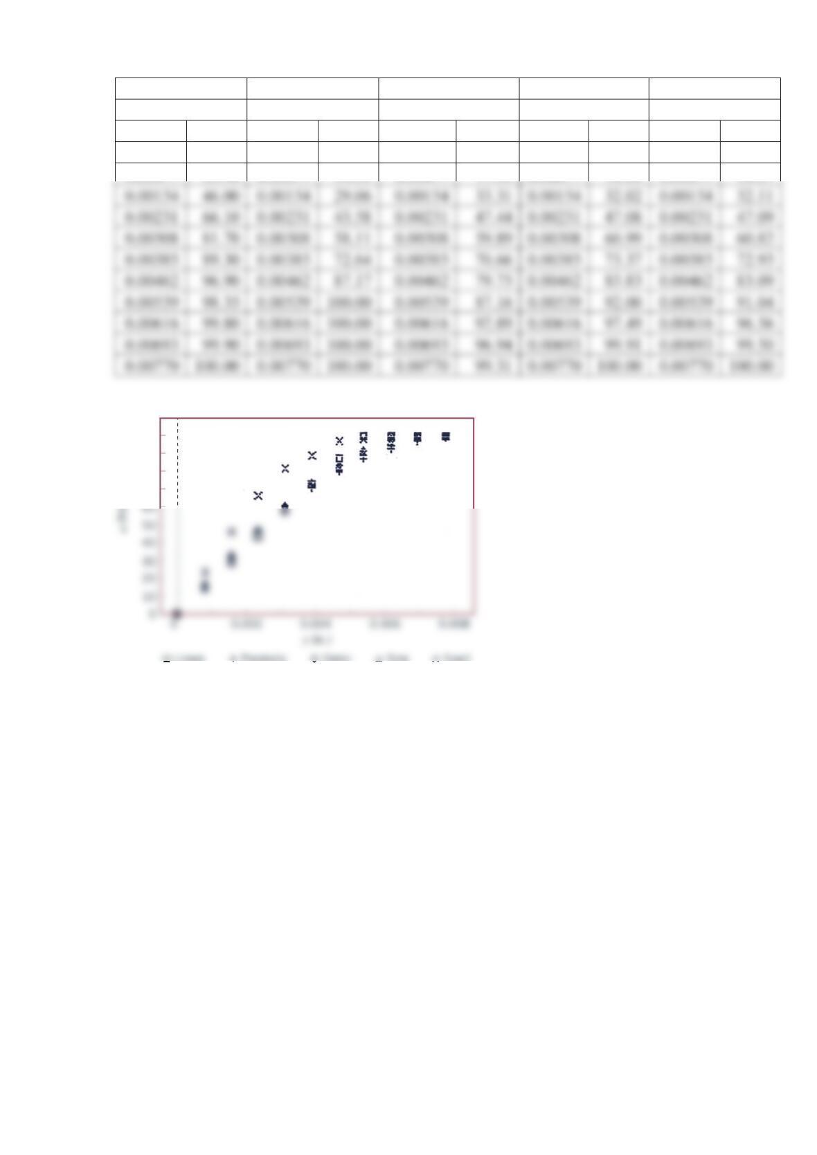
For incompressible flow 0()QQx= where
where
For example, 1ft at 0
d
x==
and 1.096ft at 10ft
d
x==
.
1 ft
d
(
x
)2 ft/s
U
=
2 ft/s
x
1,06
1,08
1,10
d vs x
Problem 9.20
A smooth, flat plate of length 6m=
and width 4m
b
= is placed in water with an upstream
velocity of 0.5 m s
U
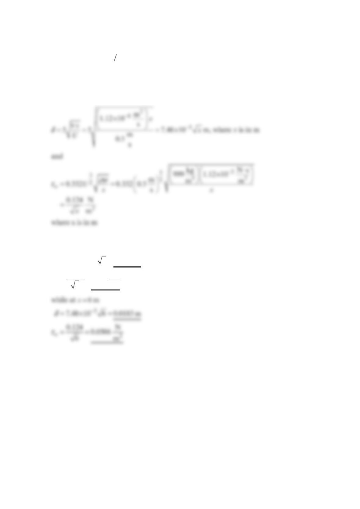
=. Determine the boundary layer thickness and the wall shear stress at
the center and the trailing edge of the plate. Assume a laminar boundary layer.
Solution 9.20
Thus, at 3mx=
3
2
7.48 10 3 0.0130
m
0.124 N
0.716
3m
w
δ
τ
−
=× =
==
τ
Problem 9.21
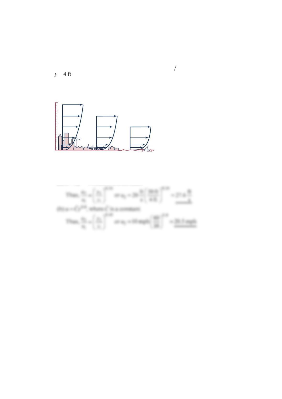
An atmospheric boundary layer is formed when the wind blows over the Earth’s surface.
Typically, such velocity profiles can be written as a power law: =n
uay
, where the constants
a
and
n
depend on the roughness of the terrain. As indicated in the figure below, typical
values are 0.40
n
= for urban areas, 0.28
n
= for woodland or suburban areas, and 0.16
n
=
for flat open country (Ref. 23). (a) If the velocity is
2
0ft s
at the bottom of the sail on your
boat ( =), what is the velocity at the top of the mast ( 30 ft
y
=)? (b) If the average
velocity is
1
0mph
on the tenth floor of an urban building, what is the average velocity on
the sixtieth floor?
Solution 9.21
(a) 0.16
uCy=, where
C
is a constant
u ~ y0.40
u ~ y0.28
u ~ y0.16
450
300
150
0
y (m)
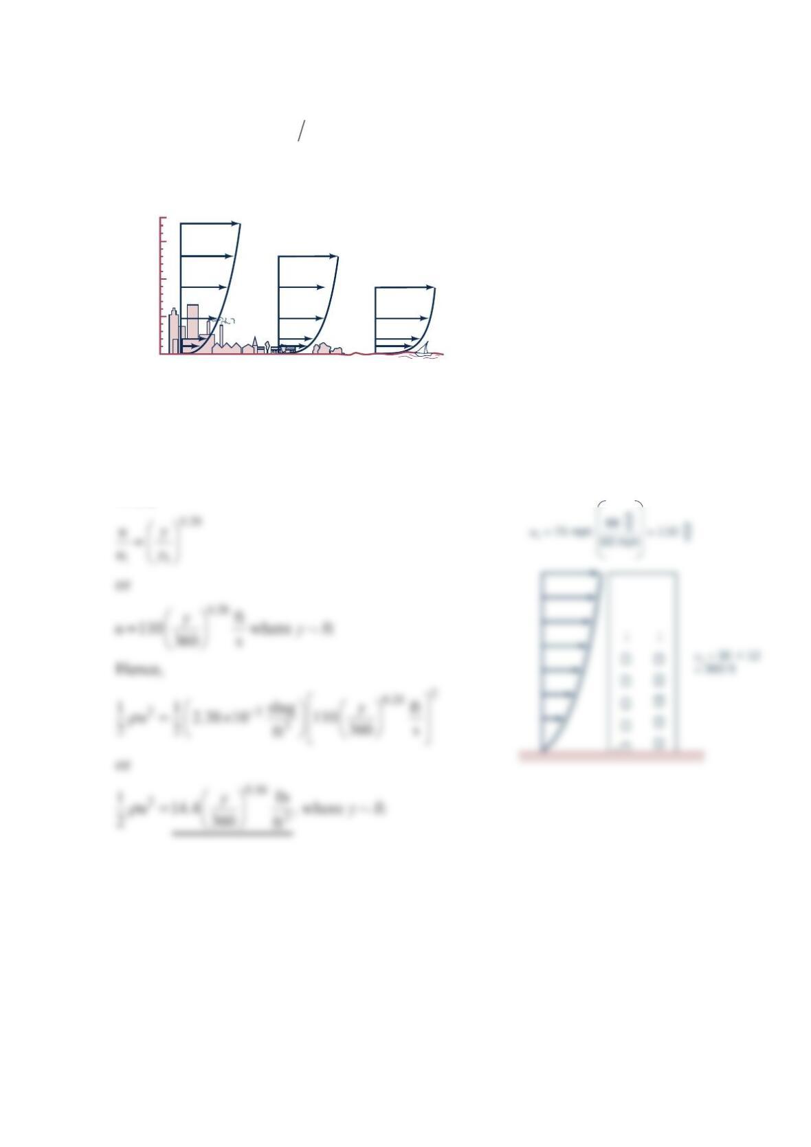
Problem 9.22
A 30-story office building (each story is
1
2ft
tall) is built in a suburban industrial park. Plot
the dynamic pressure, 2
2
u
ρ
, as a function of elevation if the wind blows at hurricane
strength
()
75 mph at the top of the building. Use the atmospheric boundary layer
information indicated in the figure below (Ref. 23).
Solution 9.22
From the figure in the problem, the boundary layer velocity profile is given by 0.28
uy∼, or
0.28
uCy=, where C is a constant.
Thus,
u ~ y0.40
u ~ y0.28
u ~ y0.16
450
300
150
0
y (m)
This is plotted in the figure below.
300
350
400
y
vs
ρ
u
2
/2
Problem 9.23
Show that by writing the velocity in terms of the similarity variable
η
and the function
()
f
η
, the momentum equation for boundary layer flow on a flat plate
2
2
uu u
uvv
xy
y
∂∂∂
+=
∂∂∂
can be written as the ordinary differential equation given by
2
0
f
ff
′′′ ′′
+=
with ′
==0ff
at
η
=0 and 1
f
′
→ as
η
→∞.
Solution 9.23
The governing equations are
Thus,
η
η
−
∂=− =−
∂
3
2
11
22
Uyx
xv x
and
η
−
∂=
∂
1
2
Ux
yv (3)
so that
Thus, using Eqs. (4) and (5), we see that Eq. (1) is satisfied for any function
()
η
f.
1
η
and
11
23 3 2
22
2
uU f U U
ff
vx y vx y vx
y
η
′′
∂∂ ∂
′′′ ′′
′
== =
∂∂
∂
(7)
Thus, using Eqs. (2.1), (6), and (7) with Eq. (2), we obtain
which simplifies to:
′′′ ′′
−=20fff
From Eq. (2.1), the boundary conditions at =0y (i.e.,
η
=0) become
()
′
==00uUf
and
Problem 9.24
Integrate the Blasius equation ( ′′′ ′′
+=20fff ) numerically to determine the boundary layer
profile for laminar flow past a flat plate. Compare your results with those of Table 9.1
Laminar Flow along a Flat Plate (the Blasius Solution).
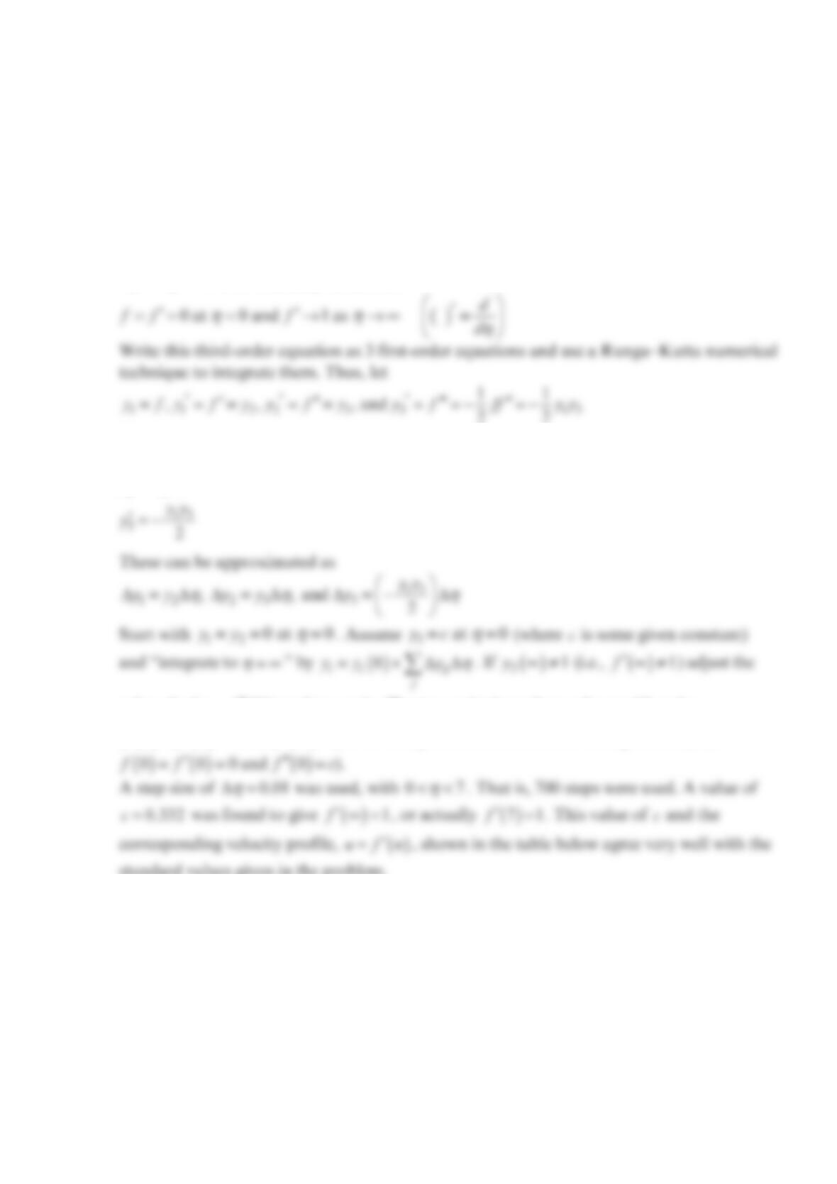
Solution 9.24
Solve the following third-order differential equation by a numerical integration technique:
′′′ ′′
+=20fff with boundary conditions
That is:
12
23
y
and
y
y
y
y
′=
′=
value of c(i.e.,
()
′′ 0f) and try again. The two-point boundary value problem (i.e.,
() ()
′
==000ff and
()
1f′∞=) is solved by iteration as an initial value problem (i.e.,
standard values given in the problem.
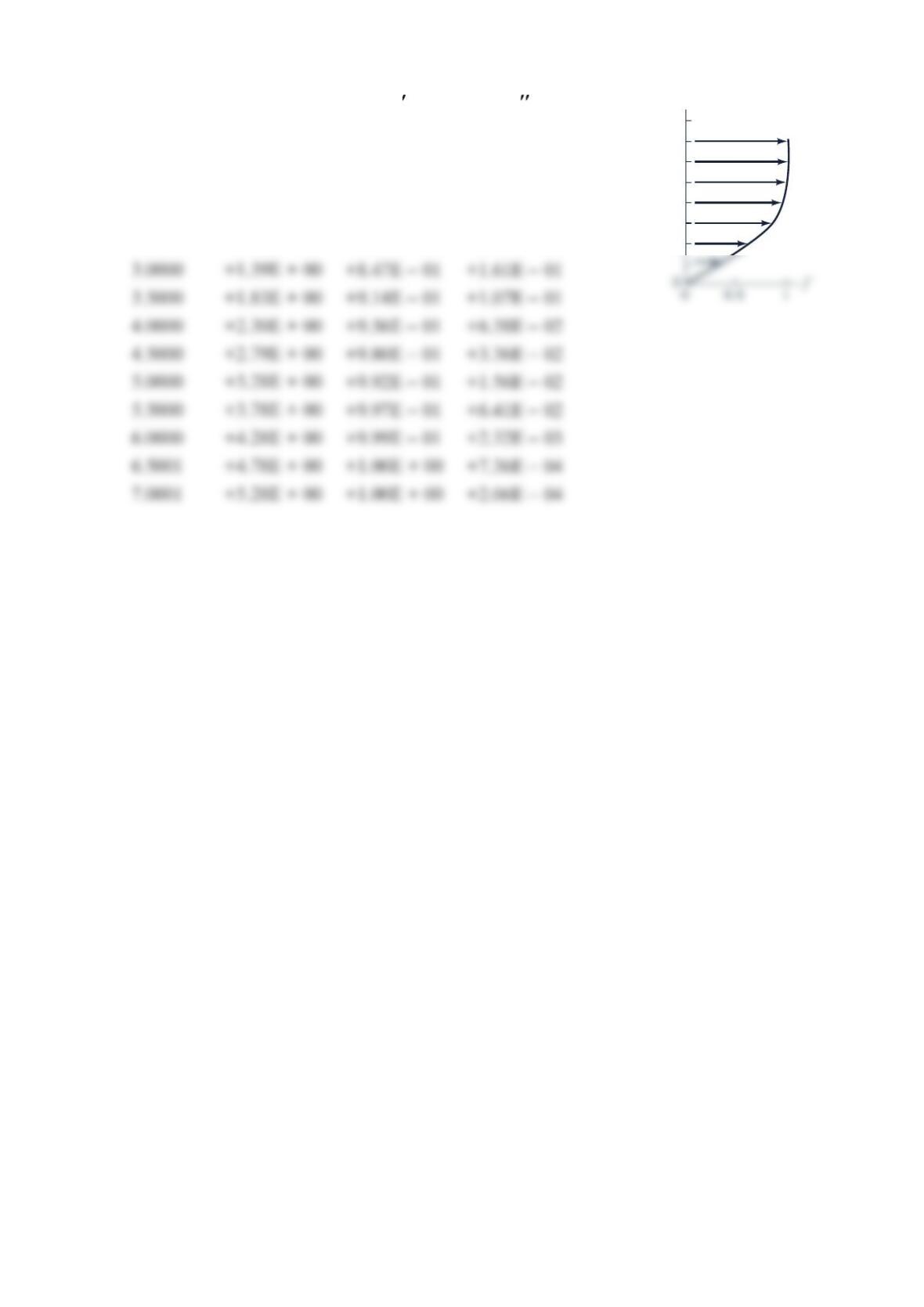
eta f f f
0.5000 +4.07E – 02 +1.66E – 01 +3.31E – 01
1.0000 +1.64E – 01 +3.30E – 01 +3.23E – 01
1.5000 +3.68E – 01 +4.87E – 01 +3.03E – 01
2.0000 +6.47E – 01 +6.30E – 01 +2.67E – 01
2.5000 +9.93E – 01 +7.52E – 01 +2.17E – 01
8
6
4
2
η
Problem 9.25
An airplane flies at a speed of 400 mph at an altitude of 10,000 ft . If the boundary layers on
the wing surfaces behave as those on a flat plate, estimate the extent of laminar boundary
layer flow along the wing. Assume a transitional Reynolds number of cr
5
x
Re 5 10=× . If the
airplane maintains its 400-mph speed but descends to sea-level elevation, will the portion of
the wing covered by a laminar boundary layer increase or decrease compared with its value
at 10,000 ft ? Explain.
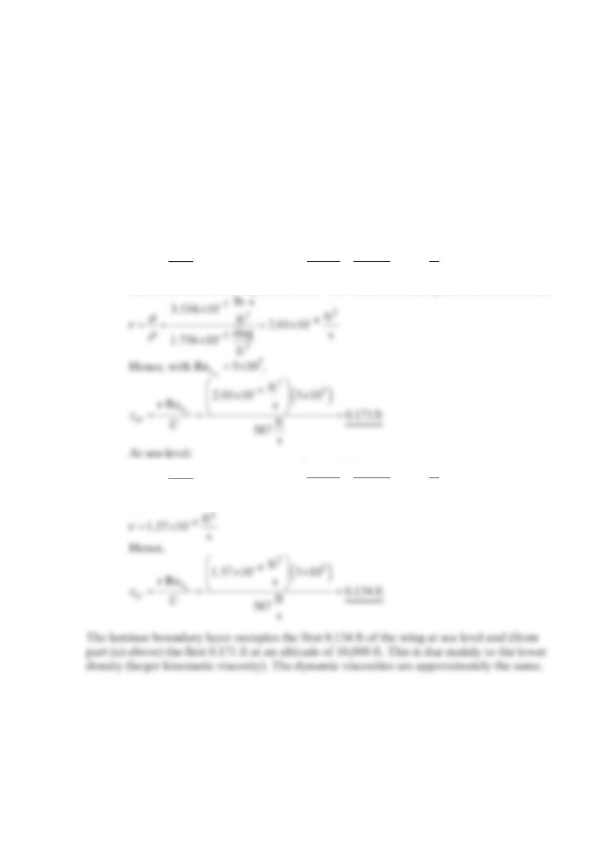
Solution 9.25
At 10,000 ft :
(a) cr
x
Re cr
Ux
ν
=, where 1 hr 5280 ft ft
400 mph 587
3600 s mi s
U
==
and from Table C.1 Properties of the U.S. Standard Atmosphere (BG/EE Units),
(b) cr
x
Re cr
Ux
ν
=, where 1 hr 5280 ft ft
400 mph 587
3600 s mi s
U
==
and
Problem 9.27
A laminar boundary layer velocity profile is approximated by
()()
δδ
=−
/
2/ /uU y y for
δ
≤y, and =uU
for
δ
>y. (a) Show that this parabolic profile satisfies the appropriate
boundary conditions. (b) Use the momentum integral equation to determine the boundary
layer thickness,
()
δδ
=.x Compare the result with the exact Blasius Solution.
Solution 9.27
(a)
()
==−
2
2
ugY Y Y
U where
δ
=
y
Y
and
()
=
=− =
20
22 2
Y
cY
so that
()
δ
==
22 30
2
15
vx vx
U
U
Problem 9.28
Choose two of the velocity profiles and corresponding boundary layer parameter formulas
presented in Table 9.2. Plot the thickness of the boundary layer and the wall shear stress
versus x for values of x from zero to the laminar–turbulent transition point. The fluid is
2
0C° water and the free-stream velocity is 10 m/s . Ask your instructor to specify which
velocity profile models you should use.
Solution 9.28
Fluid properties 3
kg
988 m
ρ
=,
ν
−
=×
2
6m
1.0 10 s
Locate transition:
Thus
δ
ν
=Ax
Ux
τ
ρ
=2
1
2
wf
CU
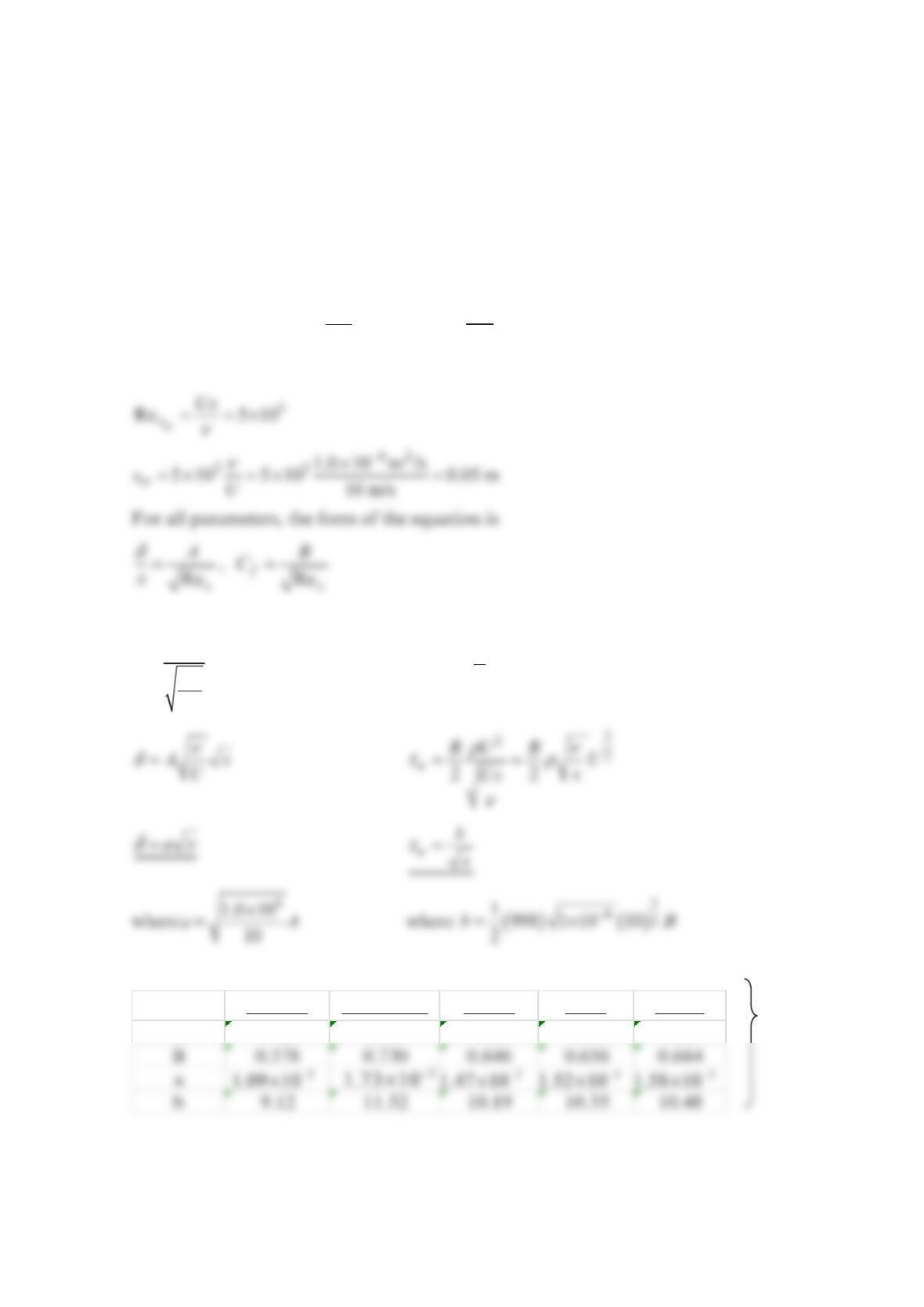
Profile Linear Parabolic Cubic Sine Exact
A 3.46 5.48 4.64 4.79 5.0
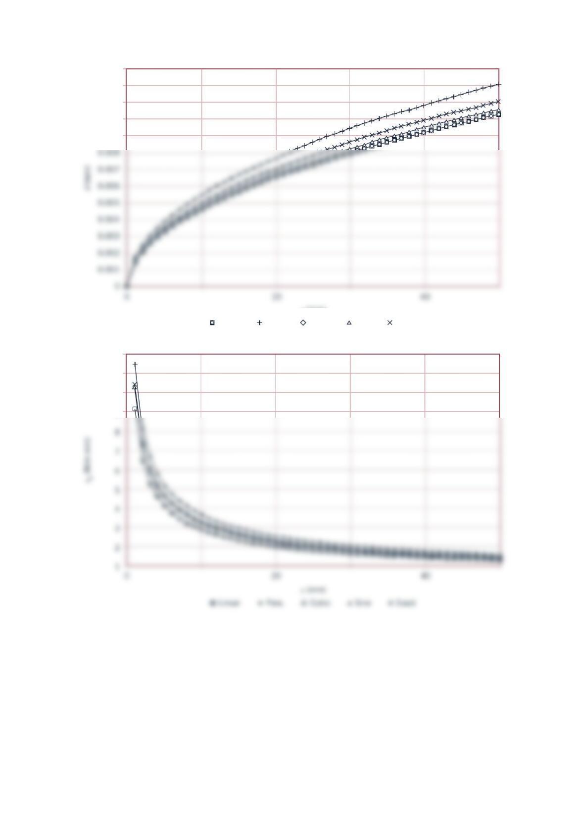
Plots below
0.013
0.012
0.011
0.01
0.009
Linear Para. Cubic Sine Exact
12
11
10
9
Boundary Layer Thickness
Wall Shear Stress
x (mm)
Problem 9.29
Air at
2
0psia
and
9
0°F
flows over a flat plate at
1
00 ft/s. Find the value of at which the
Reynolds number is . Choose three velocity profile models from Table 9.2 and plot the
velocity profiles ( vs. ) on the same axes. Ask your instructor to specify which velocity
profiles to choose.
Solution 9.29
()
2
22
33
3
lb 144 in
20 slug lb
in 1 ft 0.00305 0.0982
ft lb ft ft
1.716 10 550 R
slug °R
p
RT
ρ
== = =
⋅
×°
()
0.00154 in.A
δ
=
See following pages for tables and plot
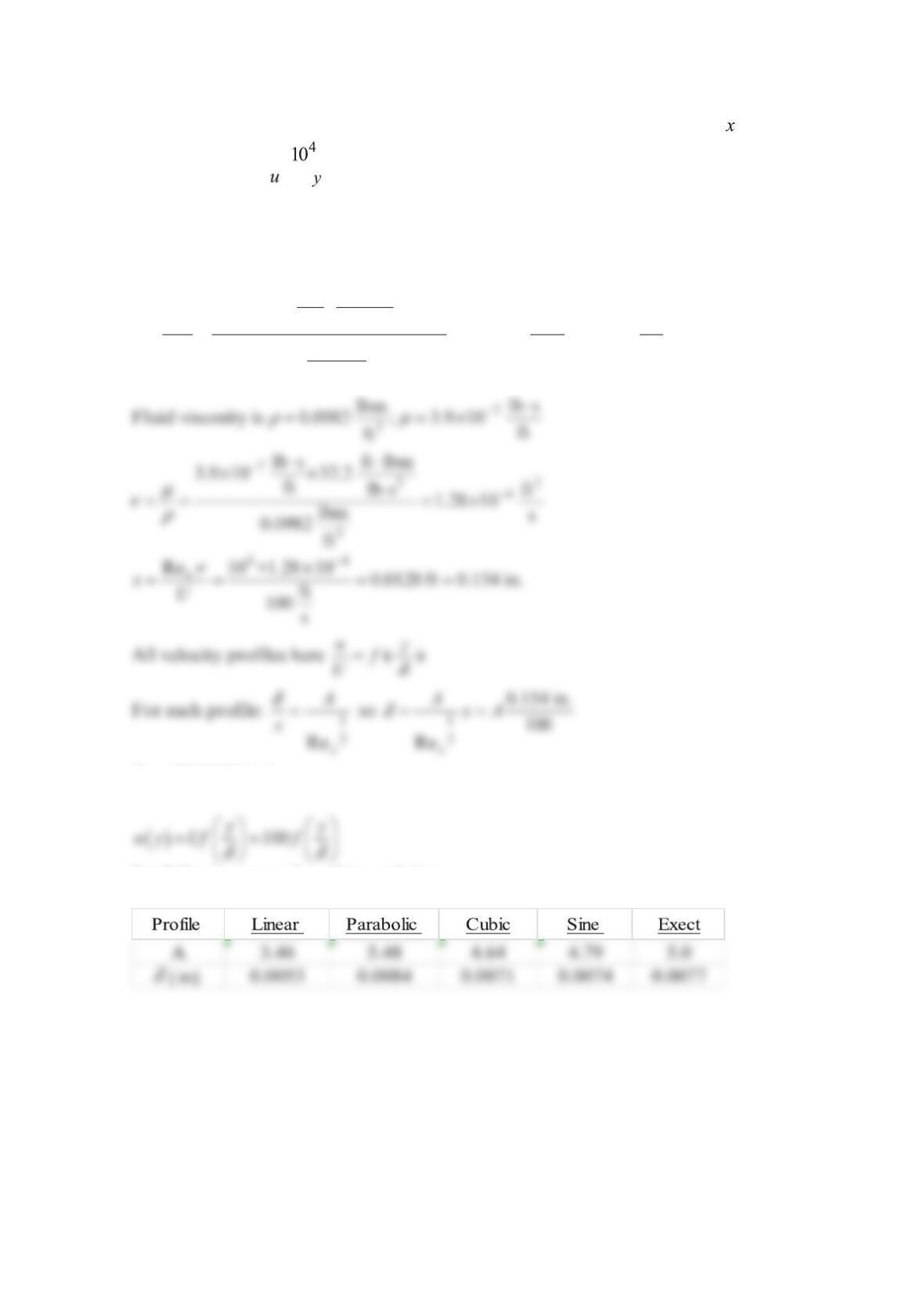
Exact Profile Linear Profile Parabolic Profile Cubic Profile Sine Profile
(delta = 0.0077) (delta = 0.0053) (delta = 0.0084) (delta = 0.0071) (delta = 0.0074)
y u y u y u y u y u
0.00000 0.00 0.00000 0.00 0.00000 0.00 0.00000 0.00 0.00000 0.00
0.00077 23.40 0.00077 14.53 0.00077 17.49 0.00077 16.20 0.00077 16.27
110
100
90
80
70
Linear Parabolic Cubic Sine Exact
Problem 9.30
A laminar boundary layer velocity profile is approximated by the two straight-line segments
indicated in the figure below. Use the momentum integral equation to determine the
boundary layer thickness,
()
δδ
=x, and wall shear stress,
()
ττ
=
ww
x. Compare these
results with those in Table 9.2 Flat Plate Momentum Integral Results for Various Assumed
Laminar Flow Velocity Profiles.
Solution 9.30
From the momentum integral equation
For ≤<
1
02
Y, =+
11
ga bY
with the constants 1
a and 1
b obtained from =2
3
g at =1
2
Y
Hence, =
2
4
3
C (2)
y
δ
δ
/2
u
U
02
U
___
3
Hence,
which upon integration gives =
10.1574C (3)
By combining Eqs. (1), (2), and (3), we obtain
Problem 9.31
A laminar boundary layer velocity profile is approximated by
()()()
34
/
2/ 2/ /uU y y y
δδδ
=− +
for
δ
≤y, and =uU
for
δ
>y. (a) Show that this profile satisfies the appropriate boundary
conditions. (b) Use the momentum integral equation to determine the boundary layer
thickness,
()
δδ
=x. Compare the result with the exact Blasius Solution.
Solution 9.31
(a) Consider =0y:
=
=
0
0
y
u
U as it must.
and
()
=−
1
1
0
1CggdY,
=
=
2
0Y
dg
CdY
Thus,