Section 9.1
Chapter 9
Section 9.1
9.1.1x(t) = 7e5t, by Theorem 9.1.1.
9.1.2x(t) = −e·e−0.71t=−e1−0.71t, by Theorem 9.1.1.
9.1.5y(t) = −0.8e0.8t, by Theorem 9.1.1.
9.1.6x dx =dt
9.1.7x−2dx =dt
−x−1=t+C
9.1.8x−1/2dx =dt
9.1.9x−kdx =dt
9.1.10 cos x dx =dt
sin x=t+C, and C= 0.
Chapter 9
9.1.11 dx
1+x2=dt
arctan(x) = t+Cand C= 0.
9.1.14 ax(t) = e−t
8270 , by Theorem 9.1.1
If Tis the half-life, then e−T
8270 =1
2or −T
8270 = ln 1
2or T=−8270 ln 1
2≈5732.
The half-life is about 5732 years.
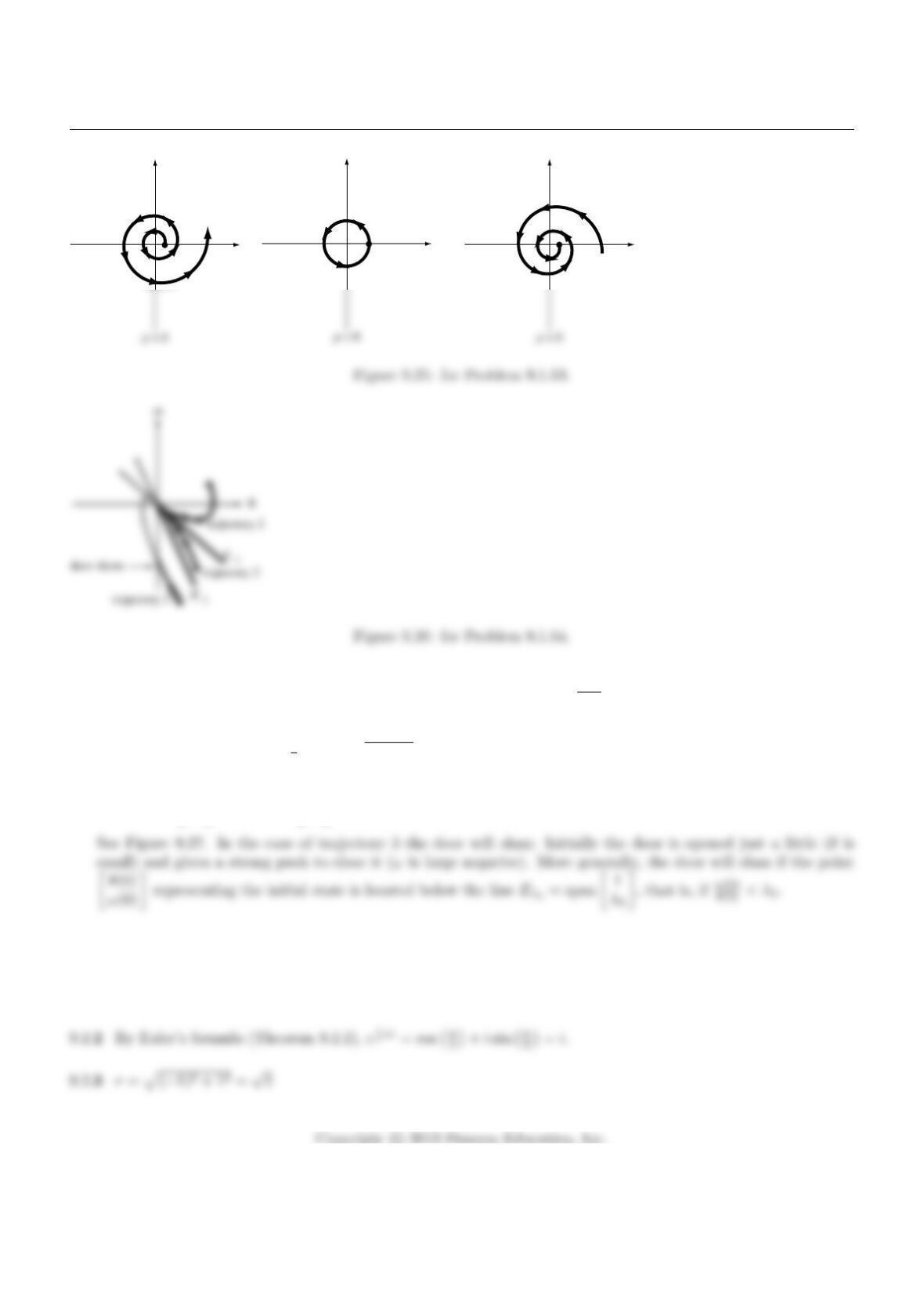
9.1.16 See Figure 9.1.
x2
9.1.17 See Figure 9.2.
9.1.18 See Figure 9.3.
412
Section 9.1
Figure 9.2: for Problem 9.1.17.
Figure 9.4: for Problem 9.1.19.
It appears that the trajectories will be circles. If we start at 1
0we will trace out the unit circle ~x(t) = cos(t)
sin(t).
We can verify that d~x
dt =−sin(t)
cos(t)equals 0−1
1 0 ~x(t) = −sin(t)
cos(t), as claimed.
413
Chapter 9
(1, 0)
x2
x1
Figure 9.6: for Problem 9.1.21.
9.1.22 We are told that d~x1
dt =A~x1and d~x2
dt =A~x2. Let ~x(t) = ~x1(t) + ~x2(t). Then d~x
dt =d~x1
dt +d~x2
dt =A~x1+A~x2=
A(~x1+~x2) = A~x, as claimed.
9.1.23 We are told that d~x1
dt =A~x1. Let ~x(t) = k~x1(t). Then d~x
dt =d
dt (k~x1) = kd~x1
dt =kA~x1=A(k~x1) = A~x, as
claimed.
9.1.26 λ1= 3, λ2=−2; ~v1=1
1, ~v2=−2
3, c1= 5, c2=−1, so that ~x(t) = 5e3t1
1−e−2t−2
3.
414
Section 9.1
By Theorem 9.1.3 the solution is ~x(t) = −1
5e−6t−3
2+2
5e−t1
1.
9.1.30 λ1= 0, λ2= 5, ~v1=−2
1,~v2=1
2;c1=−1, c2= 0, so that ~x(t) = −−2
1=2
−1.
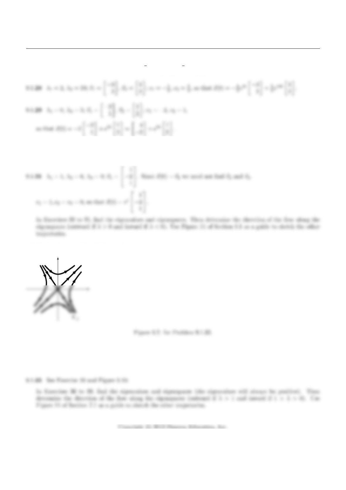
9.1.32 See Exercise 26 and Figure 9.7.
E3
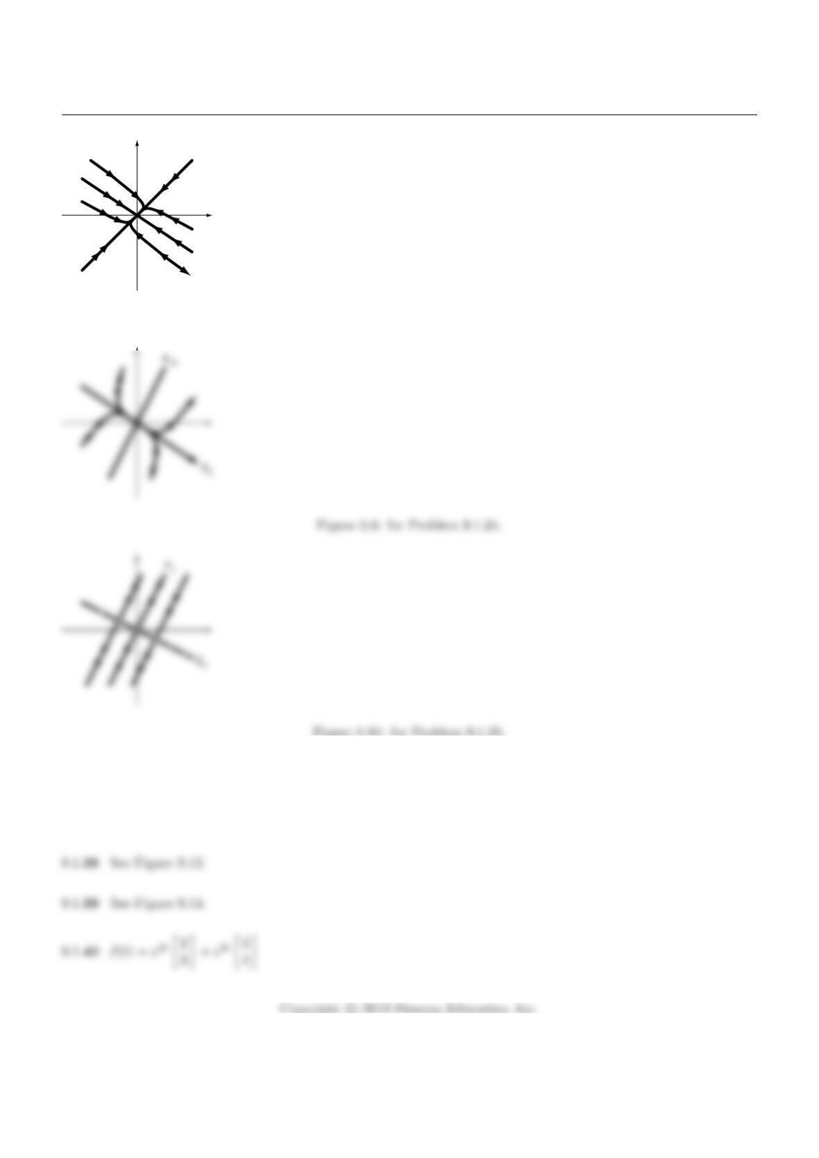
9.1.33 See Exercise 27 and Figure 9.8.
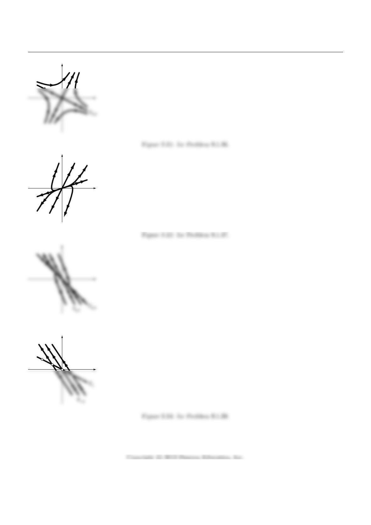
9.1.34 See Exercise 28 and Figure 9.9.
415
Chapter 9
E–1
E–6
Figure 9.8: for Problem 9.1.33.
9.1.36 See Figure 9.11.
9.1.37 See Figure 9.12.
416
Section 9.1
E1.3
E1.6
E1.1
Figure 9.13: for Problem 9.1.38.
417
Chapter 9
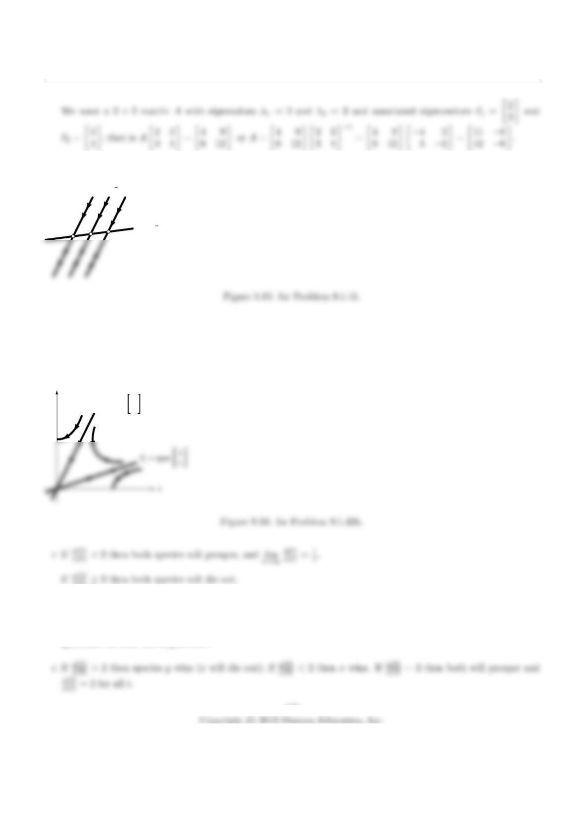
9.1.41 The trajectories are of the form ~x(t) = c1eλ1t~v1+c2eλ2t~v2=c1~v1+c2eλ2t~v2. See Figure 9.15.
span (v1)
span (v2)
9.1.42 a The term 0.8xin the second equation indicates that species yis helped by x, while species xis hindered by
y(consider the term −1.2yin the first equation). Thus ypreys on x.
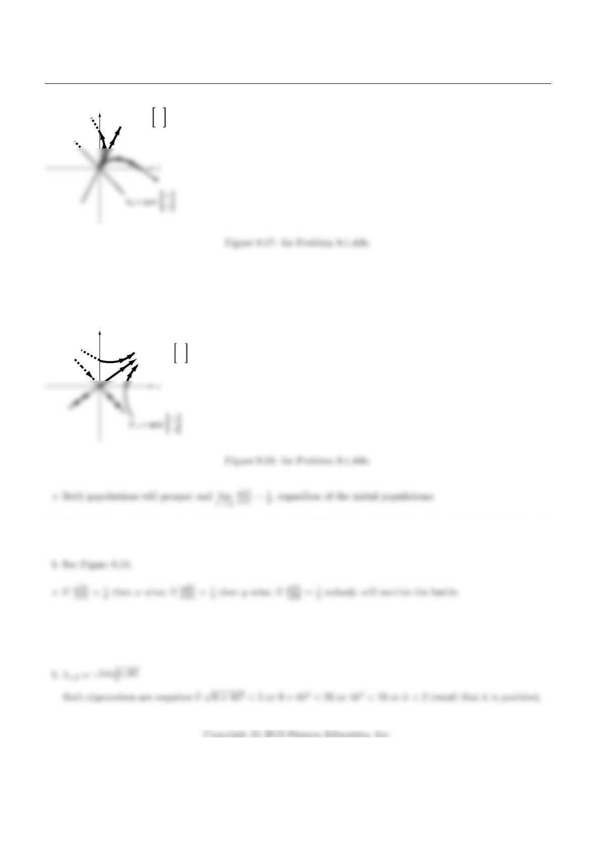
b See Figure 9.16.
E1 = span 1
2
y
x(0) ≥2 then both species will die out.
9.1.43 a These two species are competing as each is hindered by the other (consider the terms −yand −2x).
b Although only the first quadrant is relevant for our model, it is useful to consider the phase portrait in the other
quadrants as well. See Figure 9.17.
418
Section 9.1
y
E3 = span 1
2
9.1.44 a The two species are in symbiosis: Each is helped by the other (consider the terms 4yand 2x).
b See Figure 9.18.
y
E3 = span 2
1
9.1.45 a Species yhas the more vicious fighters, since they kill members of species xat a rate of 4 per time unit,
while the fighters of species xonly kill at a rate of 1.
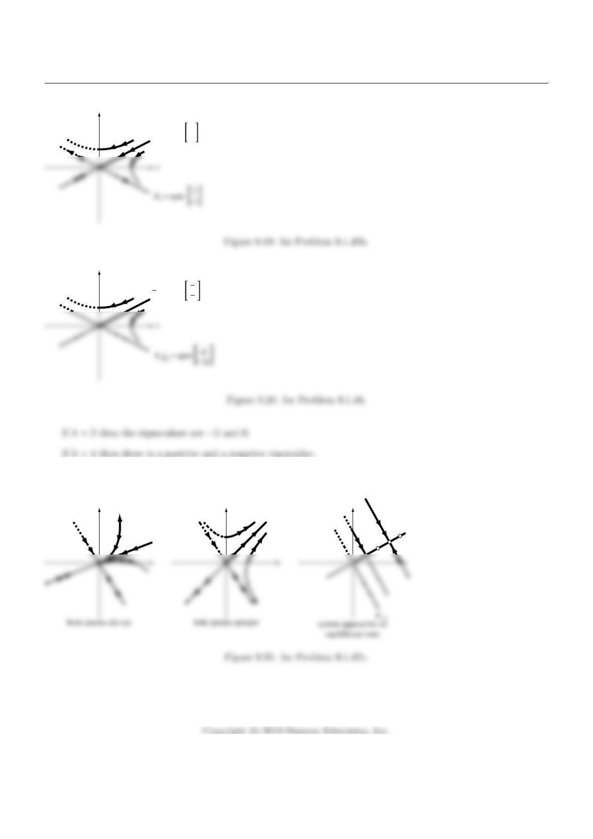
9.1.46 Look at the phase portrait in Figure 9.20.
9.1.47 a The two species are in symbiosis: Each is helped by the other (consider the positive terms kx and ky).
419
Chapter 9
y
E–2 = span 2
1
y
E–√pq = span √p
√q
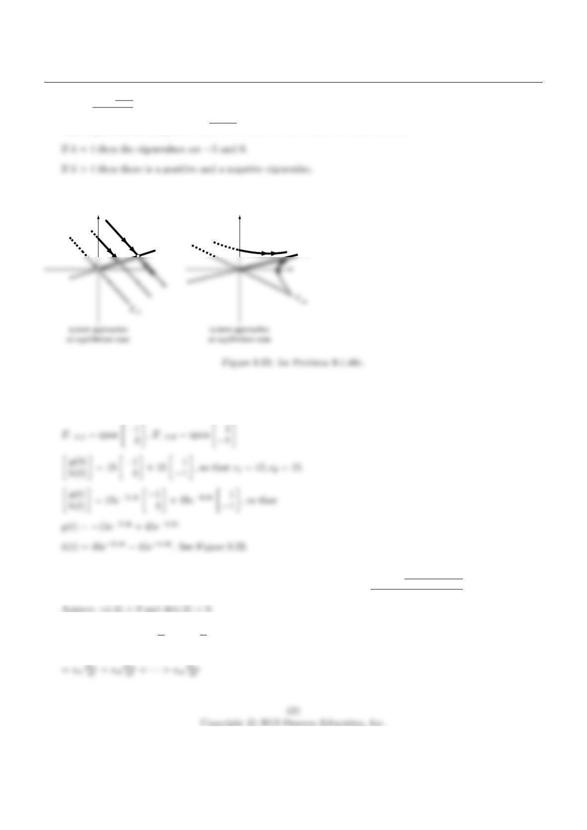
c See Figure 9.21.
E0
k = 1 k = 3 k = 2
9.1.48 a Symbiosis
420
Section 9.1
bλ1,2=−5±√9+4k
2
Both eigenvalues are negative if √9 + 4k < 5 or 9 + 4k < 25 or 4k < 16 or k < 4.
ck= 1: See corresponding figure in Exercise 47 and Figure 9.22.
E0
E1
k = 4 k = 10
9.1.49 A=−1−0.2
0.6−0.2,λ1=−0.4, λ2=−0.8
9.1.50 We want both eigenvalues λ1and λ2to be negative, so that tr(A) = λ1+λ2<0 and det(A) = λ1λ2>0.
Conversely, if tr(A)<0 and det(A)>0, then the two eigenvalues λ1,2=tr(A)±√(trA)2−4 det(A)
2are both negative.
9.1.51 ith component of d
dt (S~x) = d
dt (si1x1(t) + si2x2(t) + ···+sinxn(t))
Chapter 9
30
0
9.1.52 The solutions of d~x
dt =0 1
0 0 ~x are of the form p+qt
q, where ~x(0) = p
q, by Exercise 21. Since
λ1
0λ=λI2+0 1
0 0 , the solutions of the given system are of the form ~x(t) = eλt p+qt
q, by Exercise 24.
The zero state is a stable equilibrium solution if and only if λ < 0. The case λ= 0 is discussed in Exercise 21.
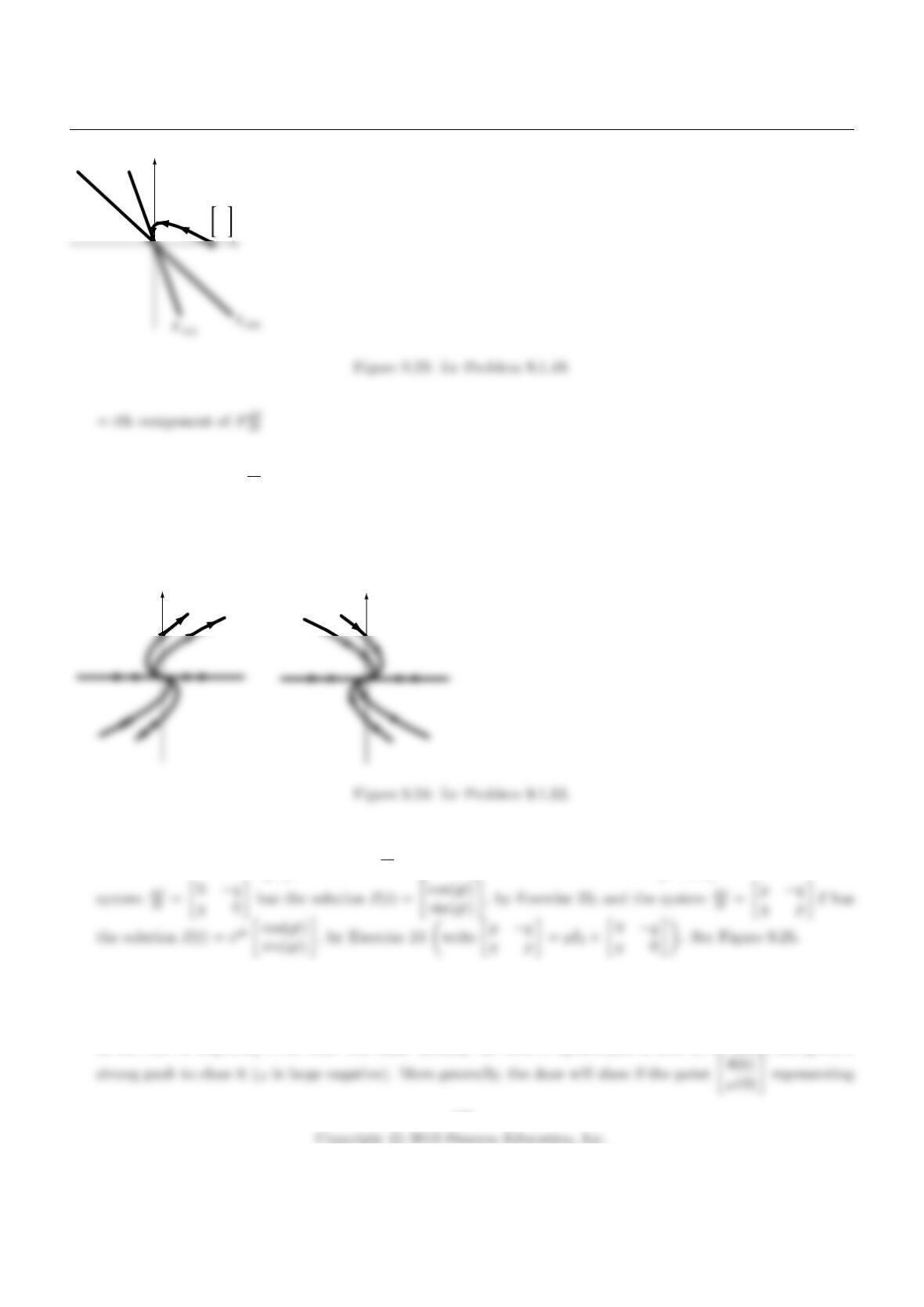
See Figure 9.24.
λ > 0 λ < 0
9.1.53 For the initial value 1
0, the system d~x
dt =0−1
1 0 ~x has the solution ~x(t) = cos(t)
sin(t), by Exercise 20; the
9.1.54 A=0 1
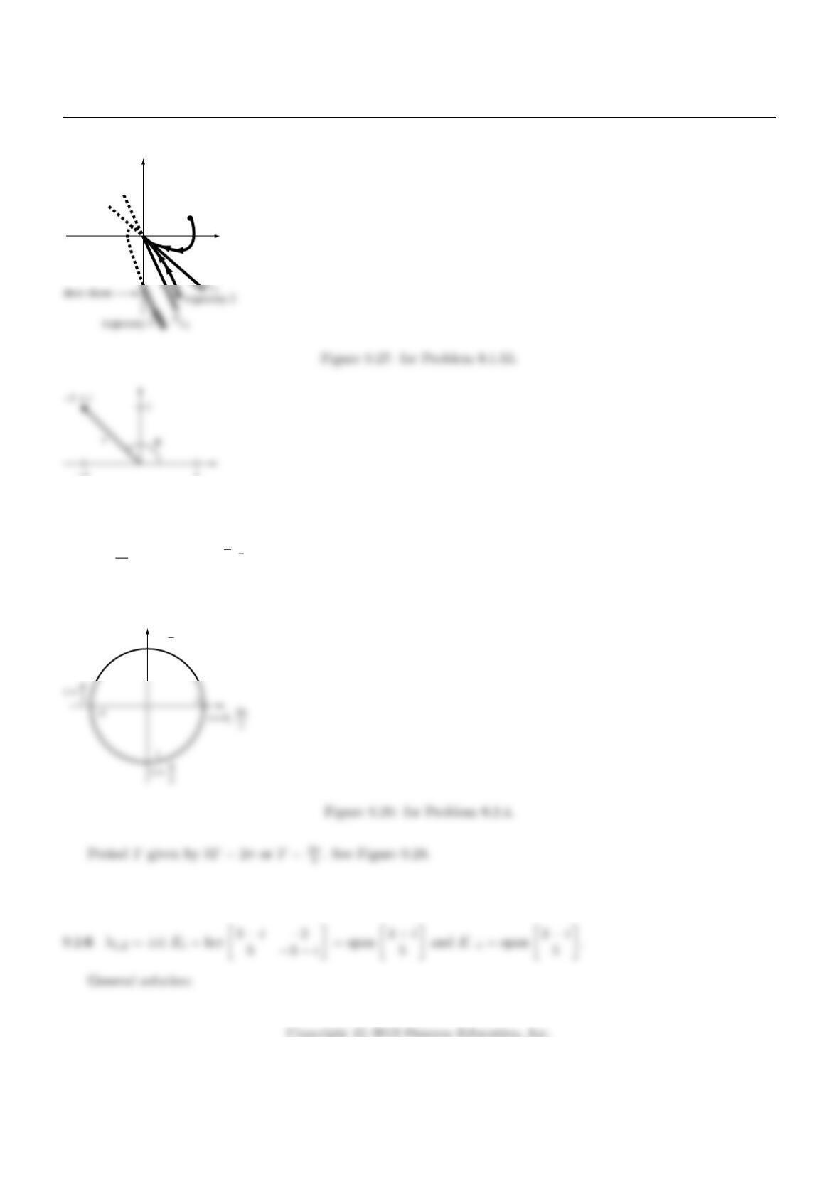
−2−3, λ1=−1, λ2=−2; ~v1=1
−1and ~v2=1
−2. See Figure 9.26.
In the case of trajectory 3 the door will slam: Initially the door is opened just a little (θis small) and given a
422
Section 9.2
the initial state is located below the line E−2= span 1
−2, that is, if ω(0)
θ(0) <−2.
9.1.55 A=0 1
−p−q, λ1,2=1
2−q±pq2−4p; note that both eigenvalues are negative.
Eλ1= span 1
λ1and Eλ2=1
λ2.
Section 9.2
9.2.1By Euler’s formula (Theorem 9.2.2), e2πi = cos(2π) + isin(2π) = 1.
423
Chapter 9
trajectory 1
θ
ω
1–1
Figure 9.28: for Problem 9.2.3.
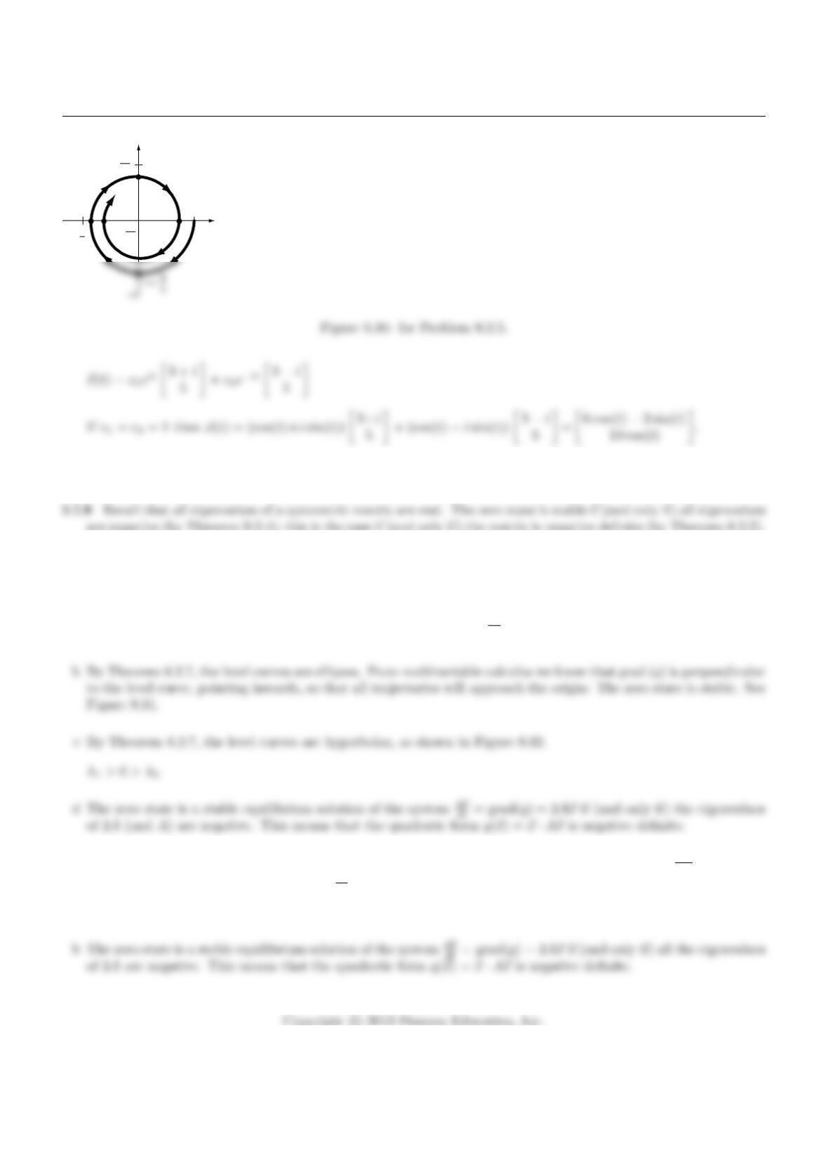
θ=3π
4, so that z=√2e3
4πi. See Figure 9.28.
9.2.4e3it = cos(3t) + isin(3t)
i
t = π
6
9.2.5e−0.1t−2it =e−0.1te−2it =e−0.1t(cos(2t)−isin(2t)) spirals inward, in clockwise direction. See Figure 9.30.
424
Section 9.2
t =
i
π
2
t =
t = 0
t = π
3π
4
t = 3π
2
1–1
9.2.7det(A) = −2, so that the zero state is not stable, by Theorem 9.2.5.
9.2.9The eigenvalues are conjugate complex, λ1,2=p±iq, and tr(A) = 2p < 0, so that pis negative. By
Theorem 9.2.4, the zero state is stable.
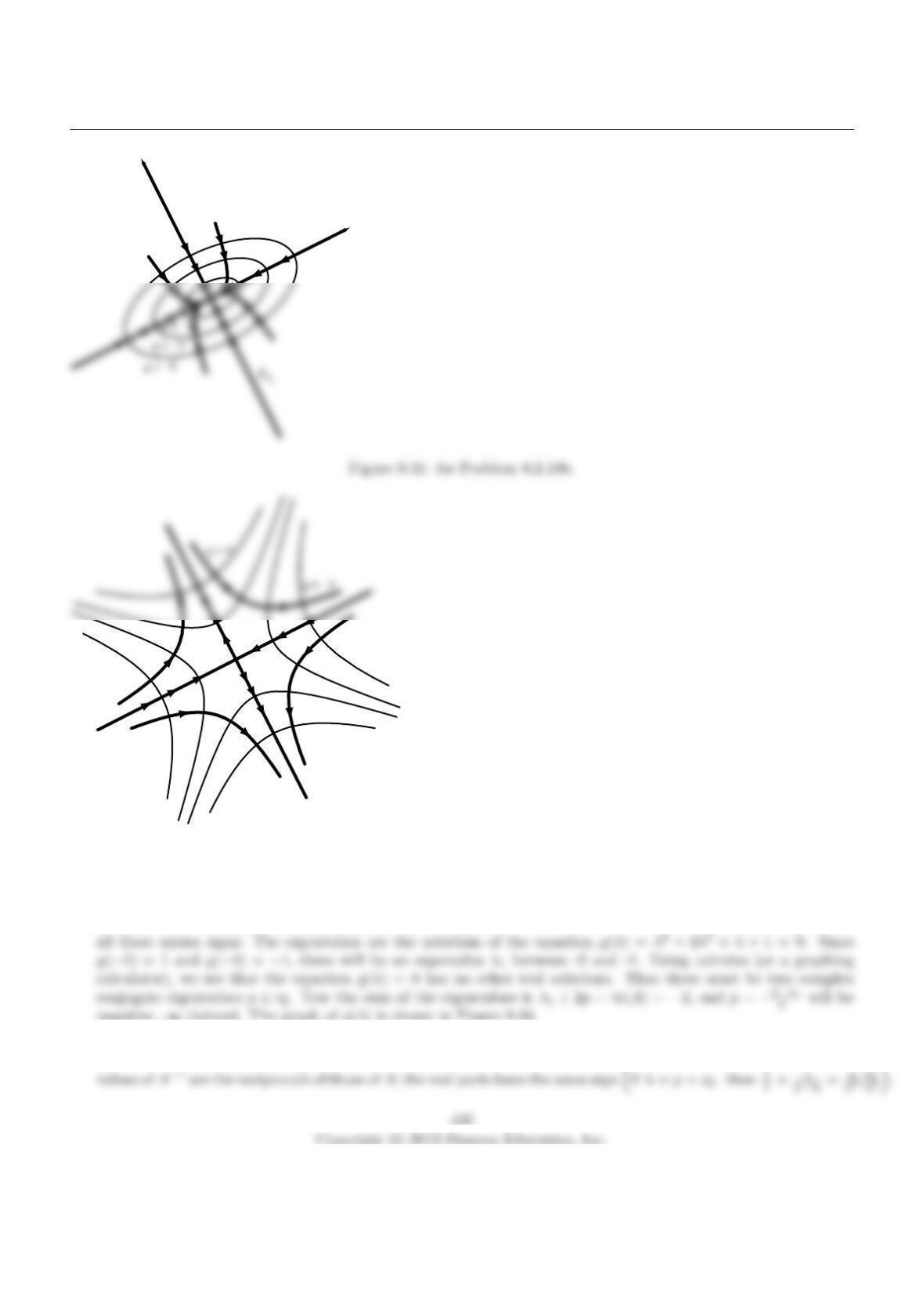
9.2.10 a The matrix of the system is 2a2b
2b2c, which is 2A, so that d~x
dt = grad(q) = 2A~x.
9.2.11 aq(~x) = 2ai1xix1+ 2ai2xix2+···+aiix2
i+···+ 2ainxixn+ terms not involving xi, so that ∂q
∂xi= 2ai1x1+
2ai2x2+···+ 2aiixi+···+ 2ainxnand d~x
dt = grad(q) = 2A~x.
The matrix of the system is B= 2A.
425
Chapter 9
Eλ1
q = –1
q = –1
q = 1
q = 1
q = –4
q = 4
Eλ1
Eλ2
Figure 9.32: for Problem 9.2.10c.
9.2.12 We will show that the real parts of all the eigenvalues are negative, so that the zero state is a stable equilibrium
solution. Now the characteristic polynomial of Ais fA(λ) = −λ3−2λ2−λ−1. It is convenient to get rid of
9.2.13 Recall that the zero state is stable if (and only if) the real parts of all eigenvalues are negative. Now the eigen-