193
transformation seems appropriate. Let
t
Y
be the natural log of sales and
Final Estimates of Parameters
Type Coef SE Coef T P
AR 1 0.5400 0.1080 5.00 0.000
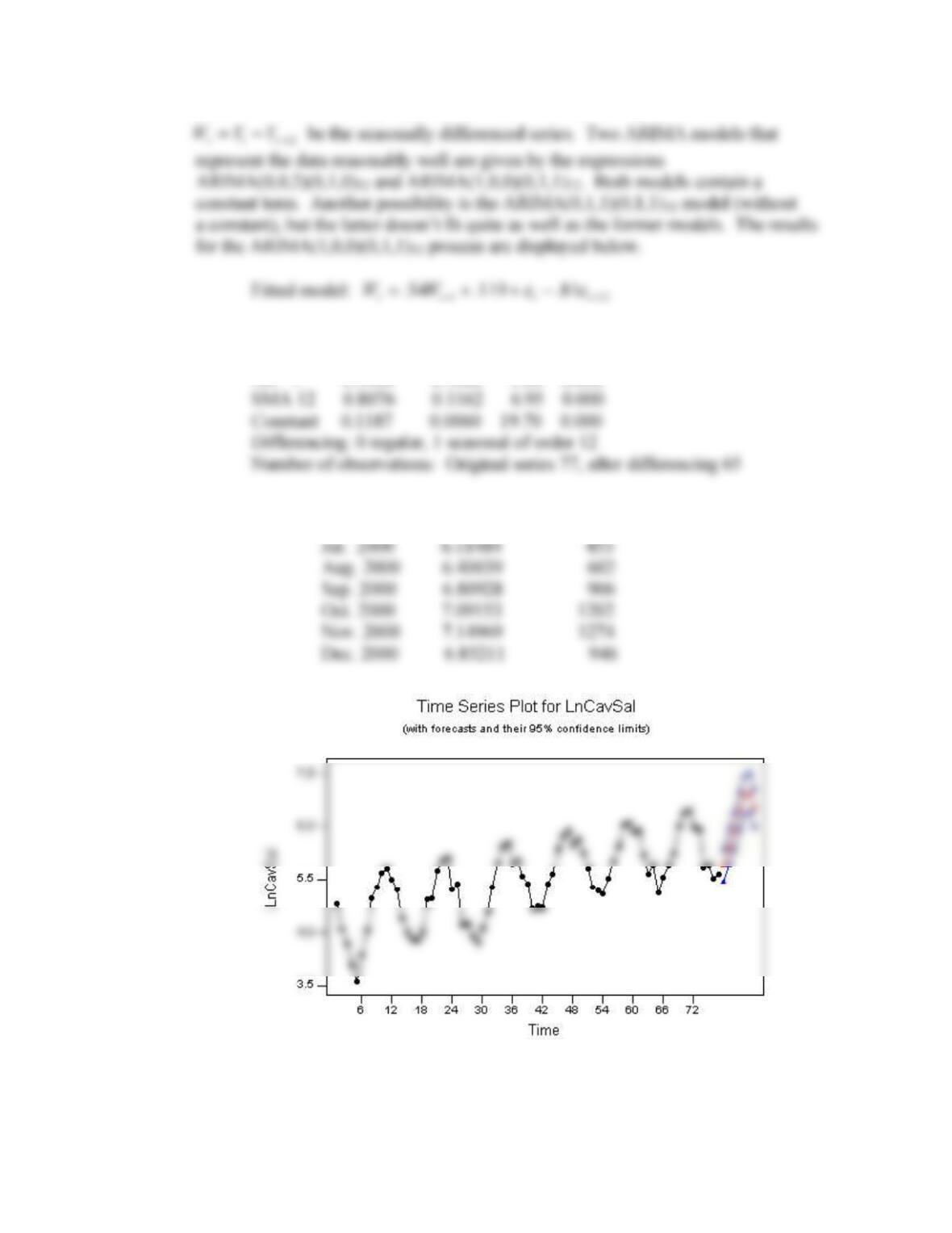
Forecasts: Date ForecastLnSales ForecastSales
Jun. 2000 5.76675 320
194
17. The variation in Disney sales increases with the level, so a log transformation
seems appropriate. Let
t
Y
be the natural log of sales and 4
ttt YYW be the
seasonally differenced series. Two ARIMA models that represent the data
reasonably well are given by the representations ARIMA(1,0,0)(0,1,1)4 and
ARIMA(0,1,1)(0,1,1)4. The former model contains a constant. The results for
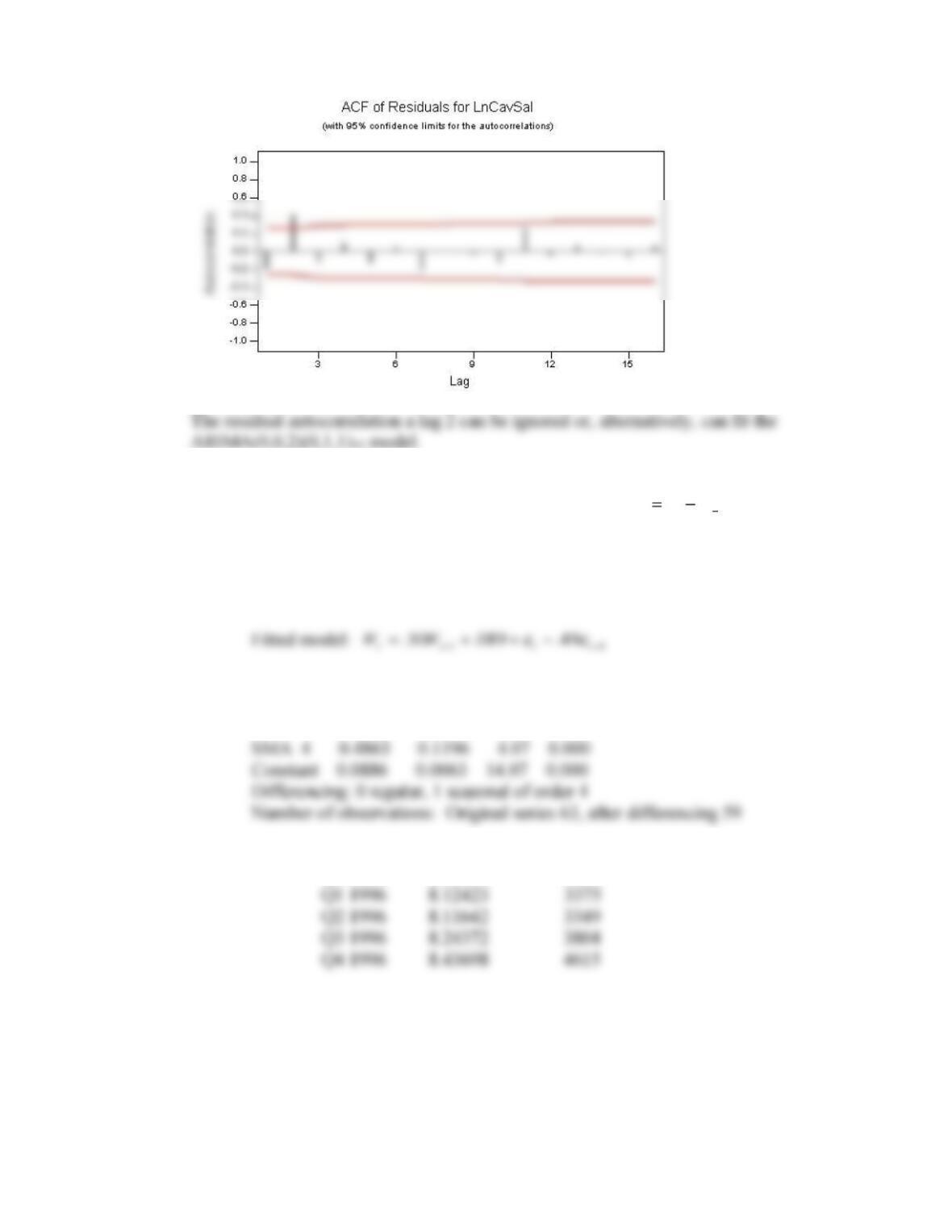
the ARIMA(1,0,0)(0,1,1)4 process are displayed below.
Final Estimates of Parameters
Type Coef SE Coef T P
AR 1 0.4991 0.1164 4.29 0.000
Forecasts: Date ForecastLnSales ForecastSales
Q4 1995 8.25008 3828
195
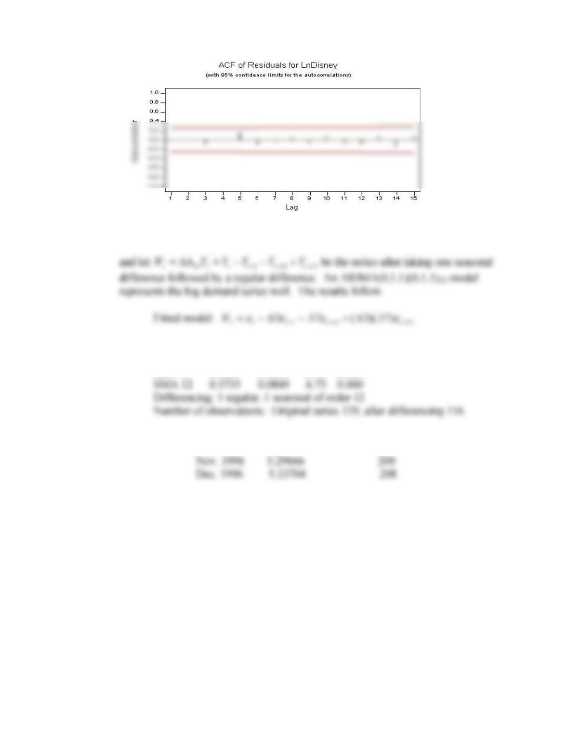
18. The data were transformed by taking natural logs; however, an ARIMA model
may be fit to the original observations. Let
t
Y
be the natural log of demand
Final Estimates of Parameters
Type Coef SE Coef T P
MA 1 0.6309 0.0724 8.71 0.000
Forecasts: Date ForecastLnDemand ForecastDemand
Oct. 1996 5.23761 188
196
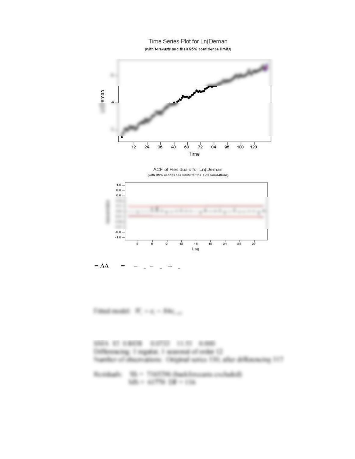
19. Let
13
12112
tttttt
YYYYYW
be the series after taking one seasonal
difference followed by a regular difference. Examination of the autocorrelation
function for
t
W
leads to the identification of an ARIMA(0,1,0)(0,1,1)12 model.
The results follow.
Final Estimates of Parameters
Type Coef SE Coef T P
Modified Box-Pierce (Ljung-Box) Chi-Square statistic
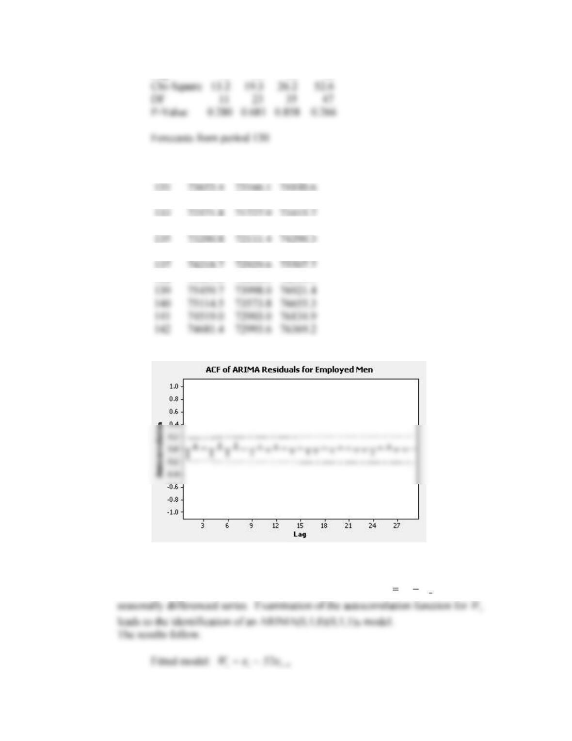
197
Lag 12 24 36 48
95% Limits
Period Forecast Lower Upper
132 73448.7 72759.7 74137.8
134 72904.3 71929.8 73878.7
136 73711.5 72518.1 74905.0
138 75021.6 73643.5 76399.7
20. The variation in Wal-Mart sales increases with the level, so a log transformation
seems appropriate. Let
t
Y
be the natural log of sales and 4
ttt YYW be the
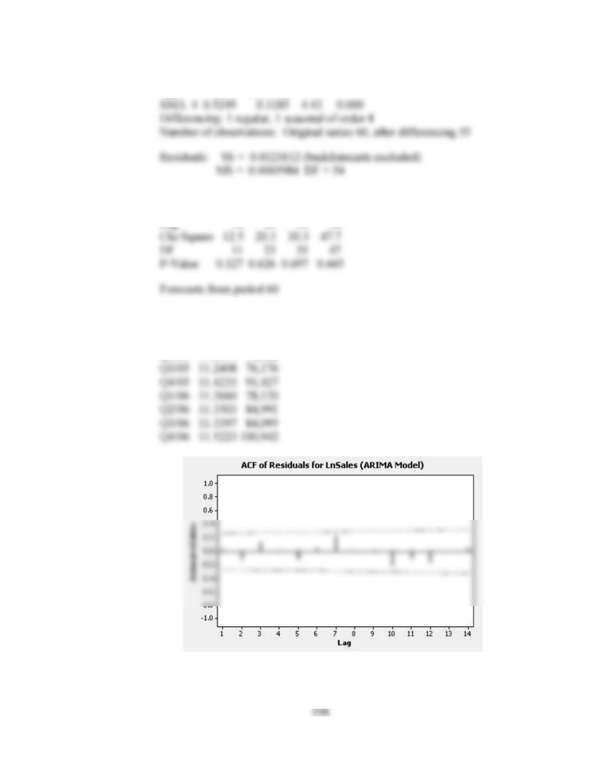
Final Estimates of Parameters
Type Coef SE Coef T P
Modified Box-Pierce (Ljung-Box) Chi-Square statistic
Lag 12 24 36 48
Forecasts
Period LnSales Sales
Q1/05 11.1671 70,764
Q2/05 11.2514 76,988
21. Autocorrelations and partial autocorrelations for number of severe earthquakes suggest
an AR(1) model.
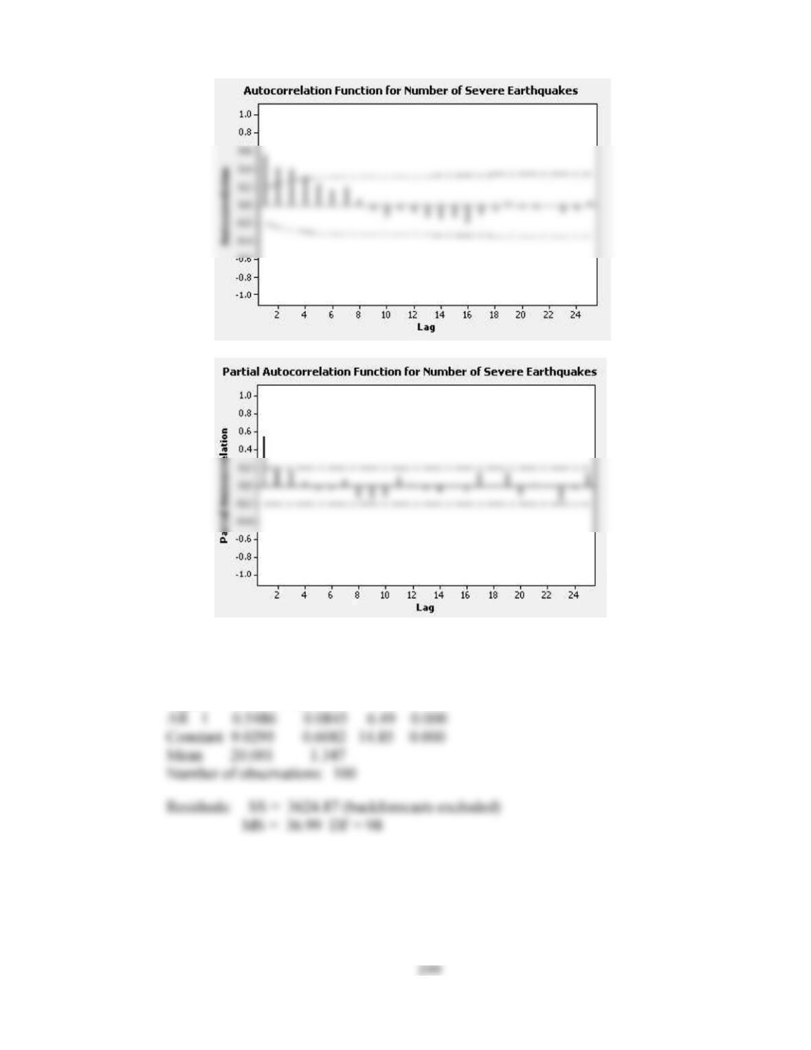
Summary of model fit and forecasts for the next 5 years follow.
Final Estimates of Parameters
Type Coef SE Coef T P
Modified Box-Pierce (Ljung-Box) Chi-Square statistic
Lag 12 24 36 48
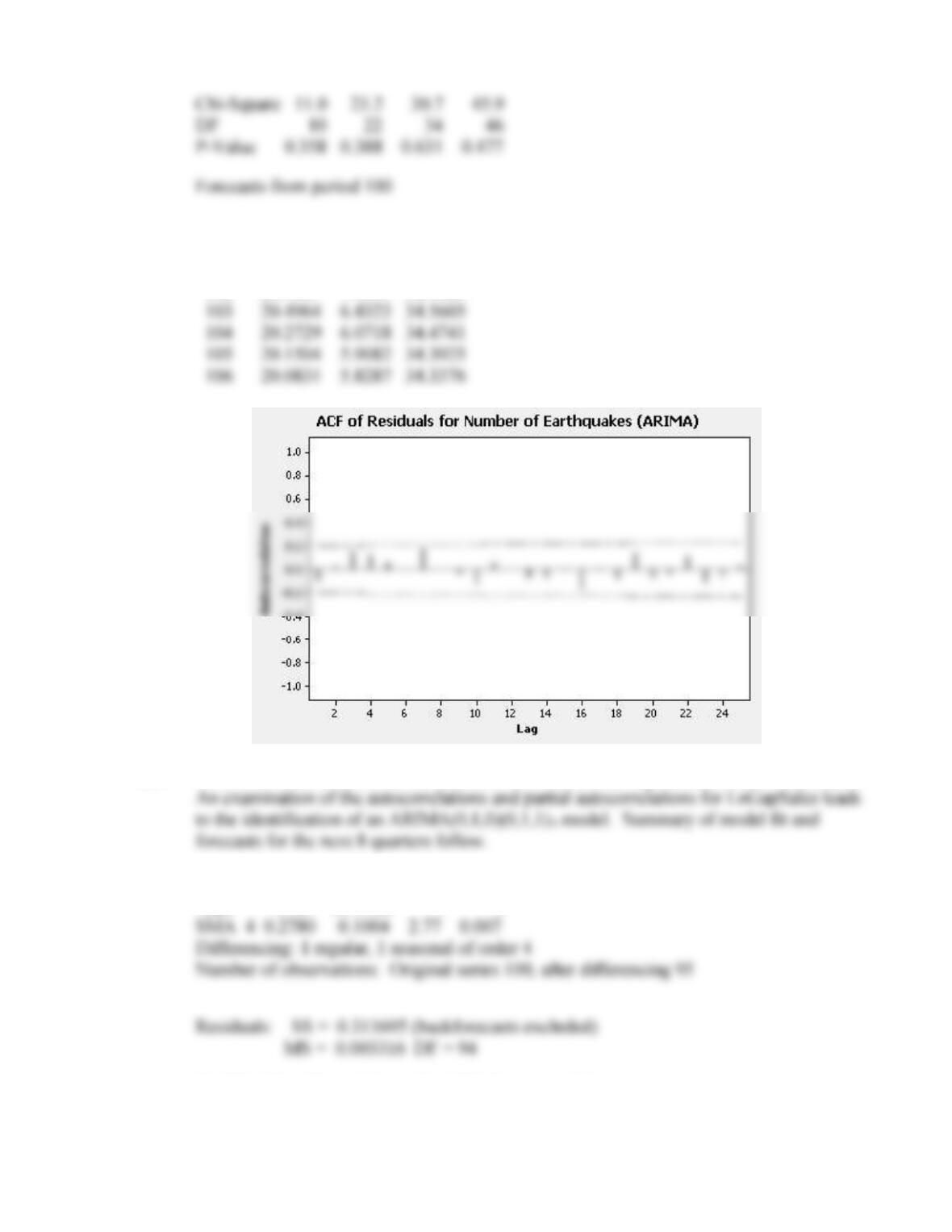
200
95% Limits
Period Forecast Lower Upper
101 21.6463 9.7236 33.5691
102 20.9037 7.3049 34.5026
22. Since the variation in the series increases with the level, a log transformation is indicated.
Final Estimates of Parameters
Type Coef SE Coef T P
Modified Box-Pierce (Ljung-Box) Chi-Square statistic
201
Lag 12 24 36 48
Period LnGapSales GapSales
102 8.23373 3,766
104 8.51475 4,988
106 8.25189 3,835
23. no Influenza A positive cases) of uneven lengths might create
identification and fitting problems for ARIMA modeling. On the other hand, a simple
CASE 9-1: RESTAURANT SALES
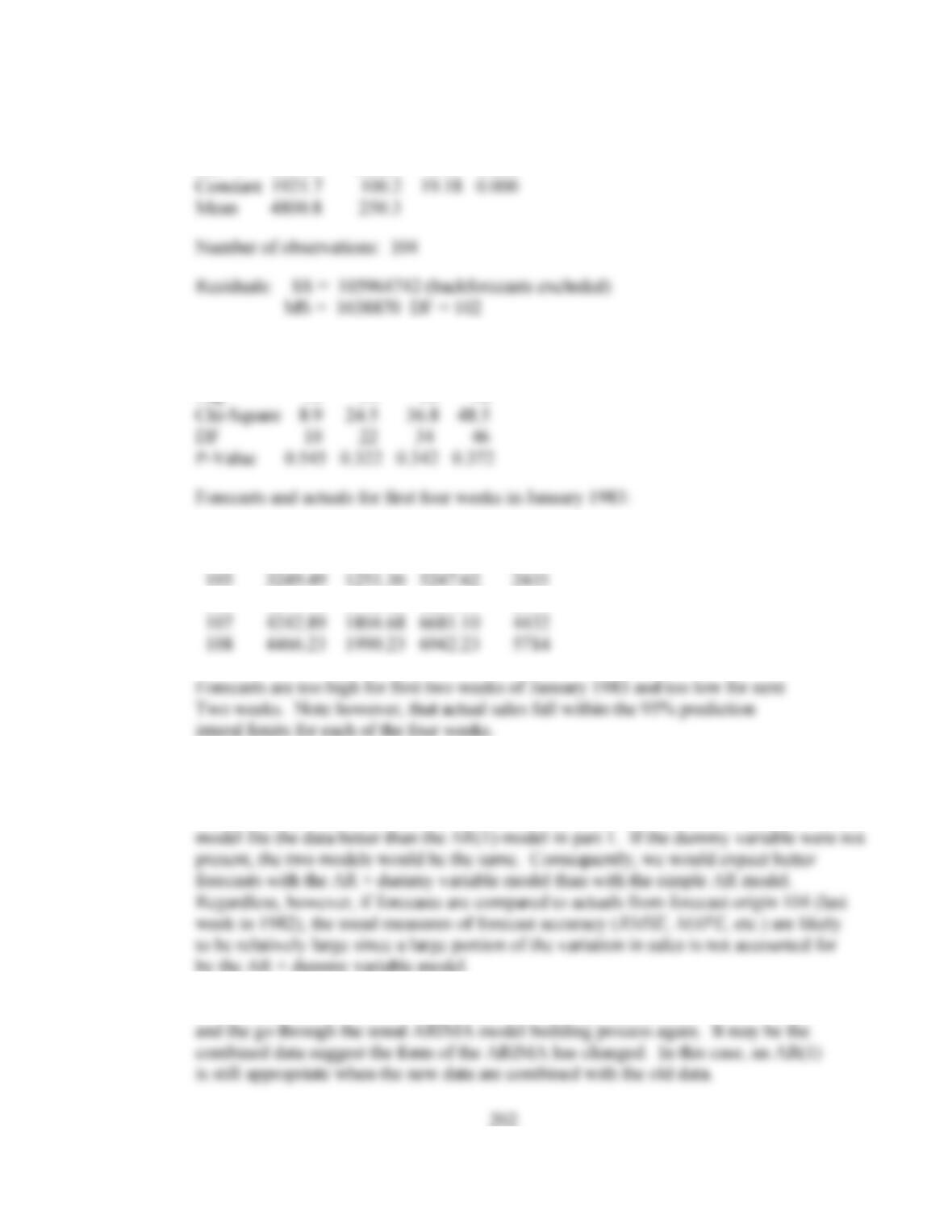
1. & 2. & 3. AR(1) model is appropriate. See summary, forecasts and actuals below.
Final Estimates of Parameters
Type Coef SE Coef T P
AR 1 0.5997 0.0817 7.34 0.000
Modified Box-Pierce (Ljung-Box) Chi-Square statistic
Lag 12 24 36 48
95% Limits
Period Forecast Lower Upper Actual
106 3870.48 1540.58 6200.38 2796
4. The best model in Chapter 8 for the original Restaurant Sales data is an autoregressive
model with an added dummy variable to represent the period during the year when
Marquette University is in session. So, because of the additional dummy variable, this
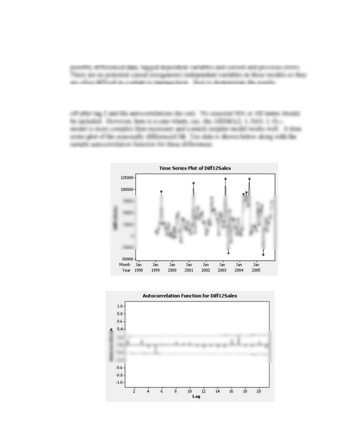
5. At the very least the parameters in the AR(1) model should be re-estimated if the
new data are combined with the old data. A better approach is to combine the data
203
CASE 9-2: MR. TUX
1. Box-Jenkins ARIMA models account for the autocorrelation in the observed series using
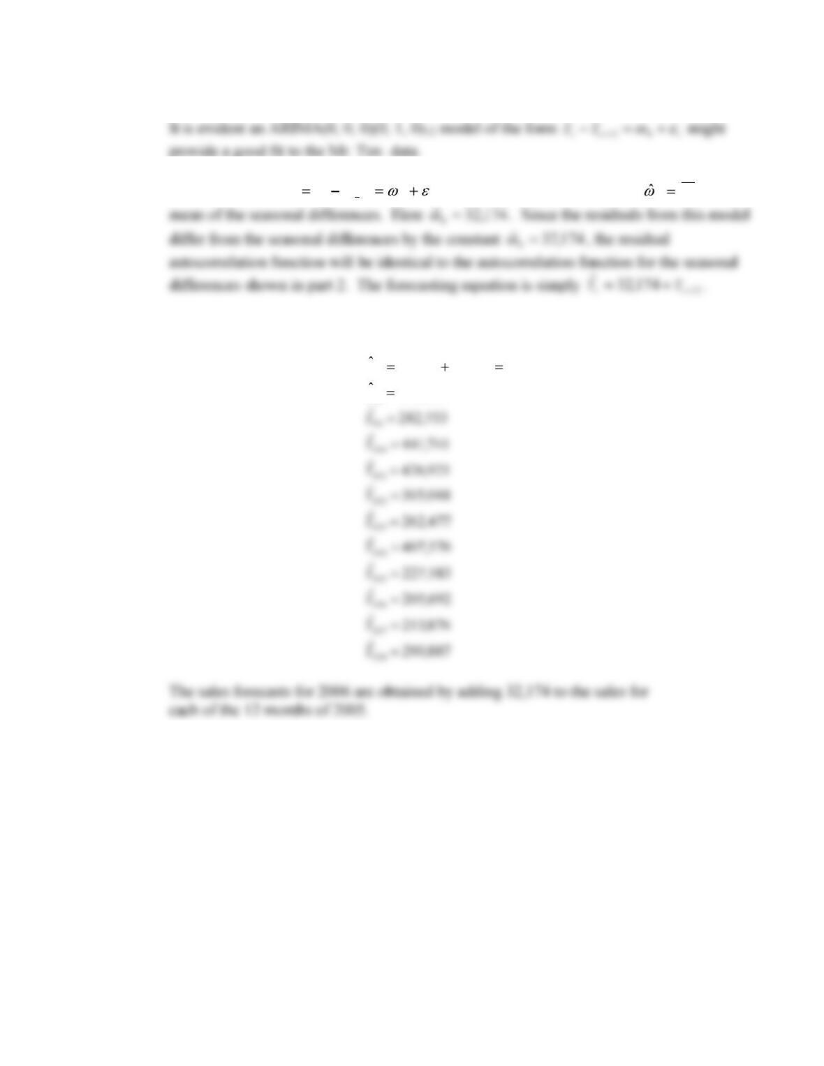
2. Autocorrelation and partial autocorrelation plots for the regular and seasonally
differenced data suggest a non-seasonal AR(2) term (the partial autocorrelations cut
204
3. To fit the model
t
ttt
YYW
012 to the Mr. Tux data, simply set
W
0, the
Setting t = 97 through t = 108, we have the forecasts for the 12 months of 2006:
104,185
217,103043,71174,32
98
97
Y
Y
CASE 9-3: CONSUMER CREDIT COUNSELING
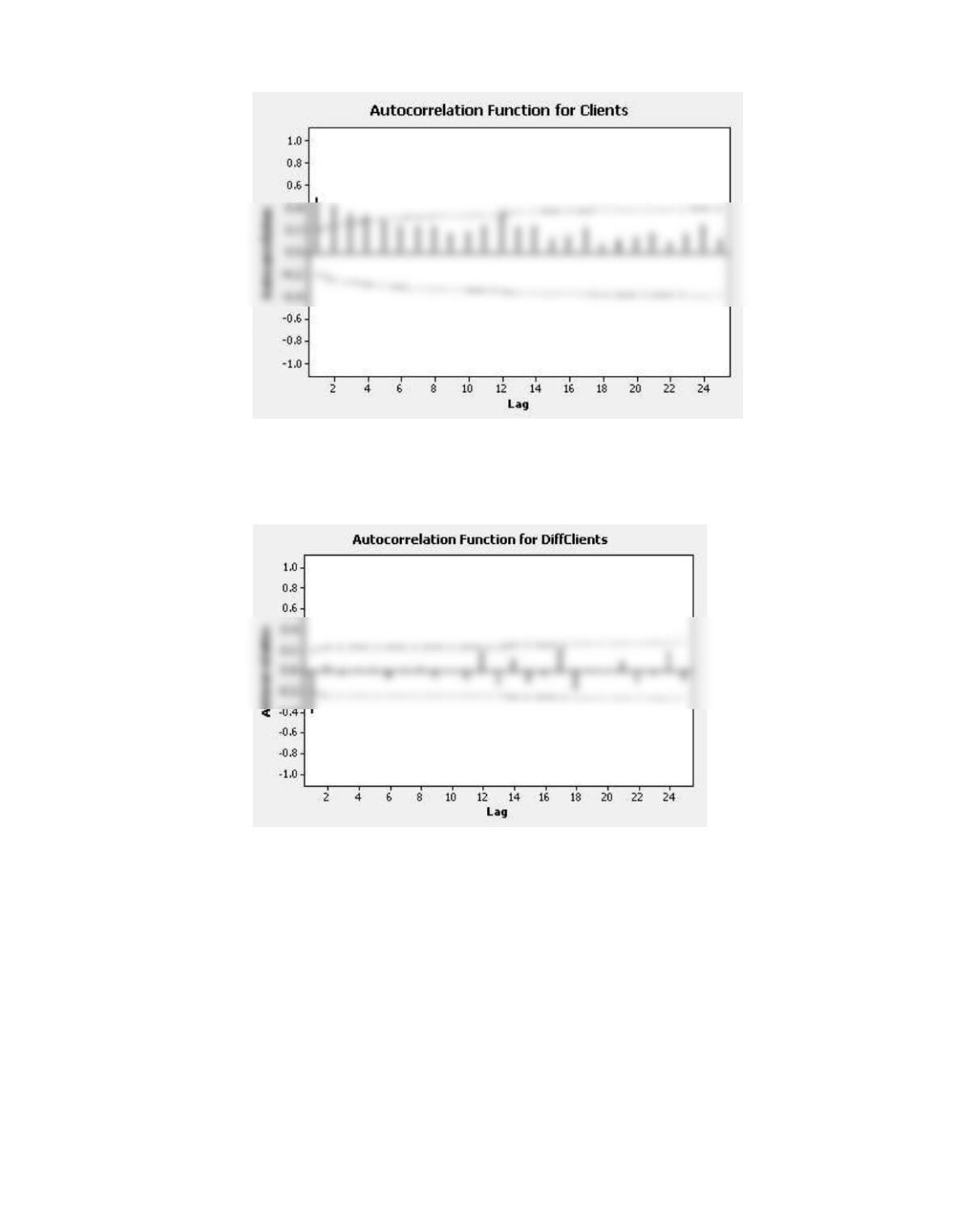
2. The autocorrelation function plot below indicates that the data are non-stationary.
The autocorrelations are slow to die out. In addition, there is a spike at lag 12 and a
smaller spike at lag 24 indicating some seasonality.
t
205
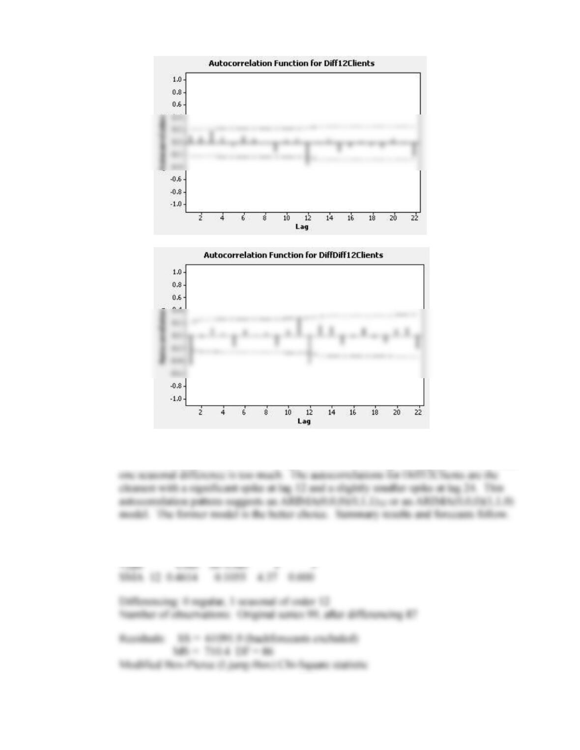
The autocorrelation functions for the differenced series (DiffClients), the seasonally
differenced series (Diff12Clients) and the series with one regular and one seasonal
difference (DiffDiff12Clients) follow.
206
Relative to the autocorrelations for DiffClients and Diff12Clients, the autocorrelations
for DiffDiff12Clients are much more pronounced, indicating one regular difference and
Final Estimates of Parameters
Lag 12 24 36 48
Chi-Square 10.9 20.3 30.8 37.4
95% Limits
Period Forecast Lower Upper
Apr 1993 123.181 70.931 175.431
May 1993 122.960 70.710 175.210
CASE 9-4: THE LYDIA E. PINKHAM MEDICINE COMPANY
1. The forecast for 1961 using the AR(2) model is 1290. The revised error
measures are:
2. The results from fitting an ARIMA(1,1,0) model, one step ahead forecasts and
actuals follow.
Final Estimates of Parameters
Type Coef SE Coef T P