
Because the problems in this chapter do not involve optimization (cost minimization principles
are not presented until Chapter 10) they tend to have a rather uninteresting focus on functional
form. Computation of marginal and average productivity functions is stressed along with a few
applications of Euler’s theorem. Instructors may want to assign one or two of these problems for
practice with specific functions, but the focus for Part (4) problems should probably be on those
in Chapters 10 and 11.
Comments on Problems
9.1 This problem illustrates the isoquant map for fixed proportions production functions.
Parts (c) and (d) show how variable proportions situations might be viewed as limiting
cases of a number of fixed proportions technologies.
9.2 This problem provides some practice with graphing isoquants and marginal productivity
relationships.
9.3 This problem explores a specific Cobb–Douglas case and begins to introduce some ideas
about cost minimization and its relationship to marginal productivities.
9.4 This problem involves production in two locations and develops the equal marginal
products rule.
9.5 This problem is a thorough examination of most of the properties of the general two-input
Cobb–Douglas production function.
9.6 This problem is an examination of the marginal productivity relations for the CES
production function.
9.7 This problem illustrates a generalized Leontief production function and provides a two-
input illustration of the general case, which is treated in the extensions.
9.8 Application of Euler’s theorem to analyze what are sometimes termed the “stages” of the
average–marginal productivity relationship. The terms “extensive” and “intensive”
margin of production might also be introduced here, although that usage appears to be
archaic.
CHAPTER 9:
Production Functions
Chapter 9: Production Functions
88
Analytical Problems
9.9 Local returns to scale. This problem introduces the local returns to scale concept and
presents an example of a function with variable returns to scale.
9.10 Returns to scale and substitution. This problem shows how returns to scale can be
incorporated into a production function while retaining its input substitution features.
9.11 More on Euler’s theorem. This problem shows how Euler’s theorem can be used to
study the likely signs of cross-productivity effects.
Solutions
9.1 a, b.
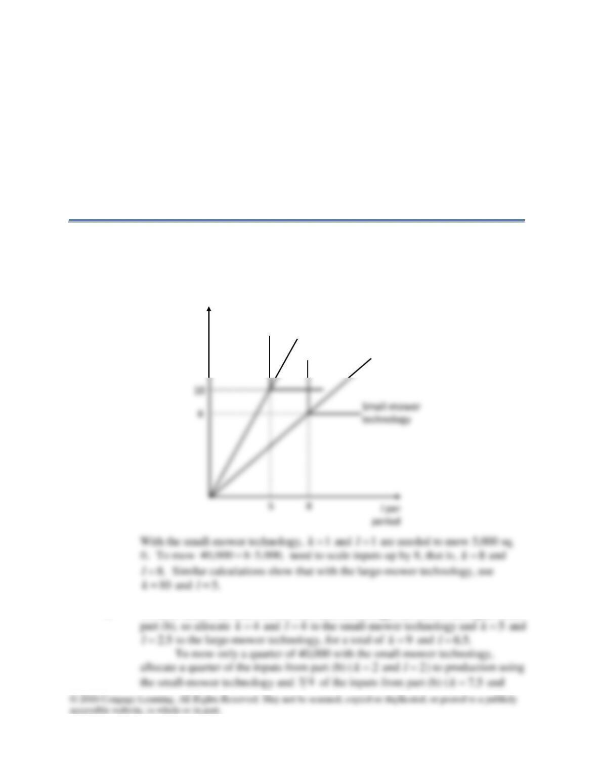
c. To mow half of the total 40,000 with each technology, use half of the inputs from
k per
period
Large-mower
technology
Chapter 9: Production Functions
89
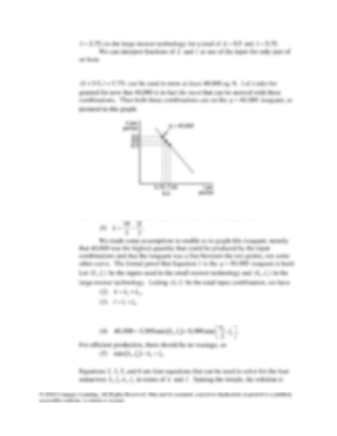
d. We know from part (c) that the combinations
( 9, 6.5)kl==
and
Assuming that the isoquant is linear, one can use the point-slope form of a line to
show that the equation for the line between the two combinations is
Total output of 40,000 is the sum of the output from technologies 1 and 2, both
Leontief:
Chapter 9: Production Functions
90
2
Substituting these solutions into Equations 5 and 6,
9.2 Given production function
22
0.8 0.2 .q kl k l= − −
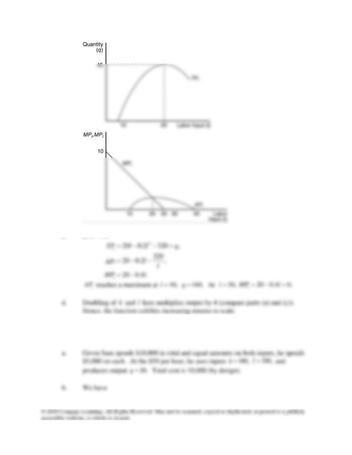
a. When k = 10, total labor productivity is
b. Marginal labor productivity is
Chapter 9: Production Functions
91
c. If
20,k=
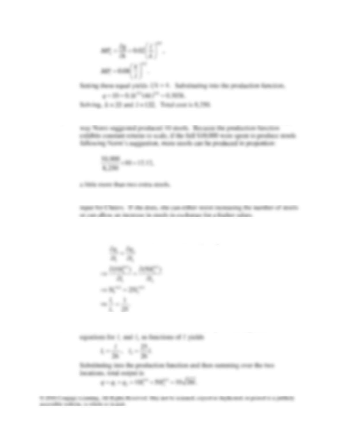
9.3 Given production function
0.2 0.8
0.1 .q k l=
Chapter 9: Production Functions
92
c. The cost savings in part (b) is 1,750. We saw in part (b) that $8,250 used in the
d. Carla’s ability to influence the decision depends on whether she provides a unique
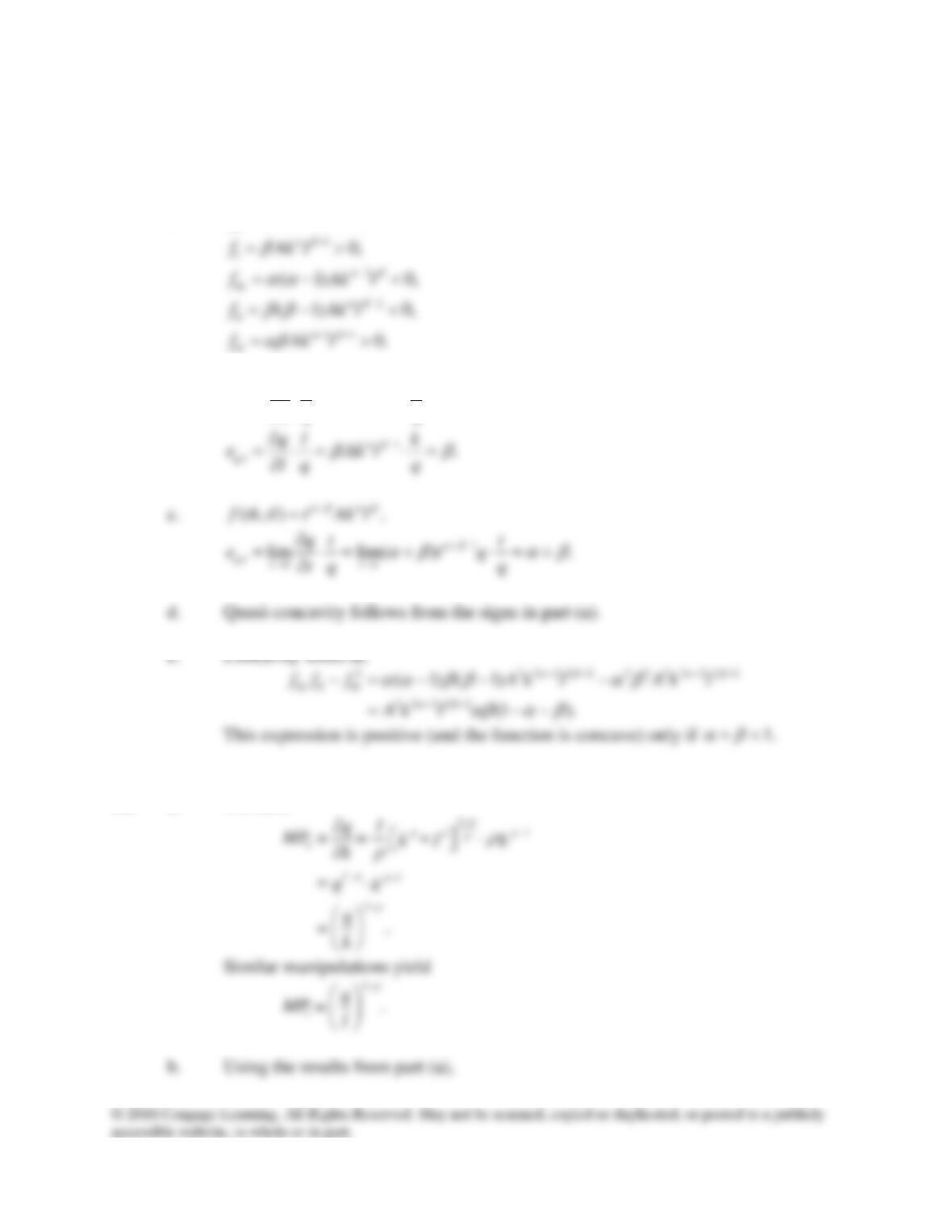
9.4 a. The firm should allocated labor such that
12
=.
ll
MP MP
2
b. In addition to the previous equation, we have
12 .l l l+=
Solving these two
Chapter 9: Production Functions
93
9.5 Given production function
.q Ak l
=
a.
10,
k
f Ak l
−
=
b.
1
,,
qk
q k k
e Ak l
k q q
−
= = =
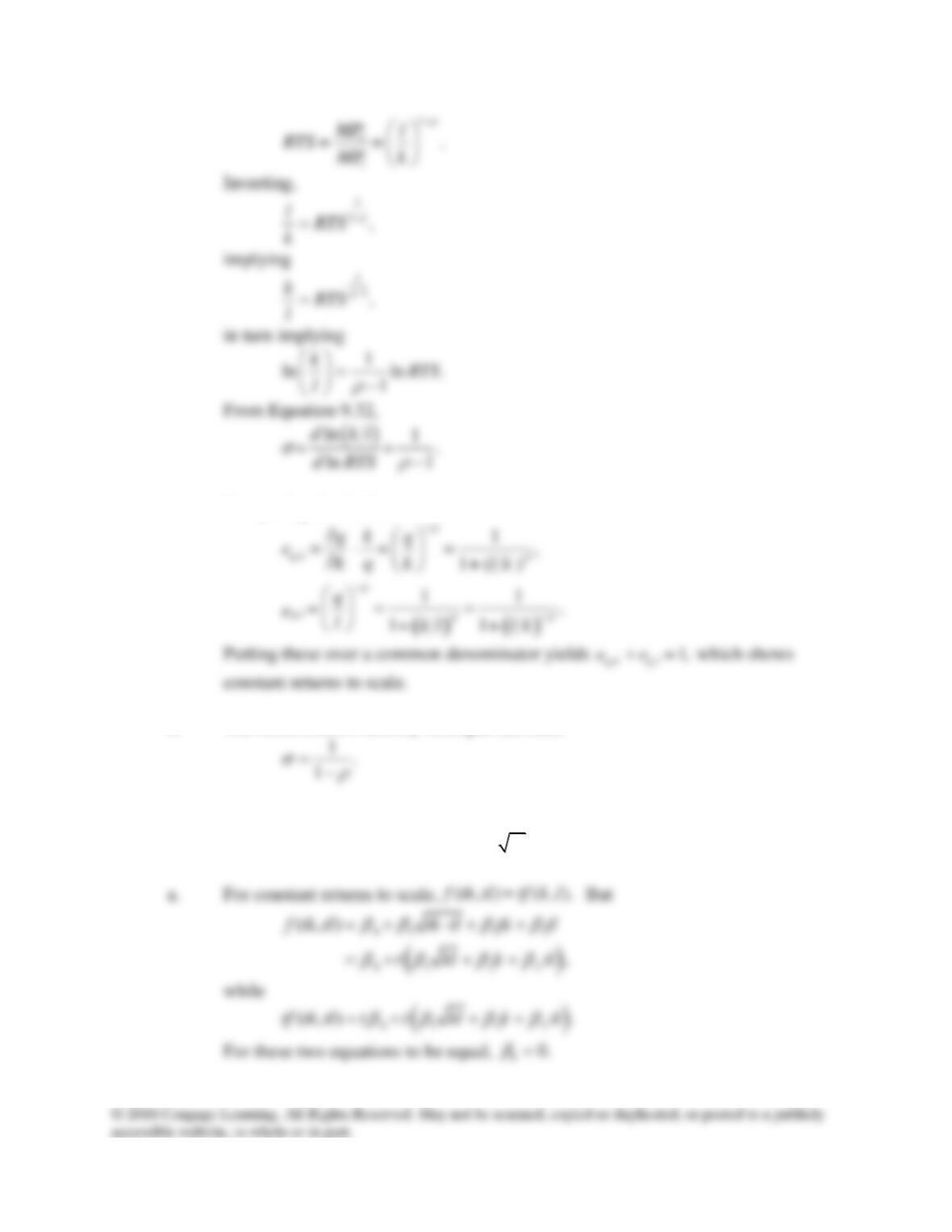
9.6 a. We have
b. Using the results from part (a),
Chapter 9: Production Functions
94
d. The result follows directly from part (a) since
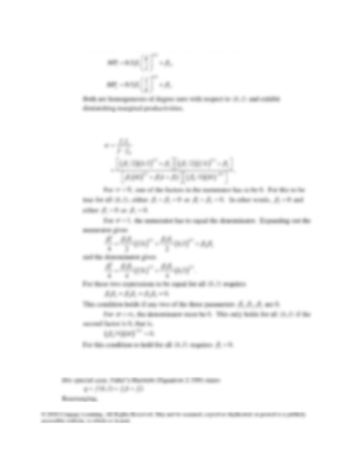
9.7 Given production function
0 1 2 3
( , ) .f k l = kl k l
+ + +
Chapter 9: Production Functions
95
b. Assume
00
=
to ensure constant returns to scale. Then
c Footnote 6 provides the key formula in the special case of constant returns to
scale:
9.8 Because
( , )q f k l=
exhibits constant returns to scale, it is homogeneous of degree 1. In
Chapter 9: Production Functions
96
Analytical Problems
9.9 Local returns to scale
a. If
( , ) ( , ),f tk tl tf k l=
then
b.
,1
( , )
lim ( , )
qt t
f tk tl t
et f tk tl
→
=
d. The intuitive reason for the changing scale elasticity is that this function has an
Chapter 9: Production Functions
97
9.10 Returns to scale and substitution
a. Let
denote the elasticity of substitution and
RTS
the marginal rate of technical
substitution associated with
.F
Then
Chapter 9: Production Functions
98
can be applied to show the elasticity of substitution for
f
equals 1. Since
F
is
just
f
scaled by the exponent
,ab+
F
the preceding results imply that the elasticity
The formula in Equation 1 can be used to show that the elasticity of substitution
for this
f
is
9.11 More on Euler’s theorem
b. Using Young’s theorem, we have
12 21.ff=
For
2n=
and
1,k=
the above
expression becomes
Chapter 9: Production Functions
99
scale, increasing one input must increase the marginal product of the other input.
If
1,k
1,k
c. Under the assumption of diminishing marginal productivity,
0
f
for
1,…, .in=
we have
i
=
Hence, returns to scale will be determined by
12 n
k
= + + +
. Further,

Chapter 9: Production Functions
100