CHAPTER 9 │ CORRELATION AND REGRESSION 373
23.
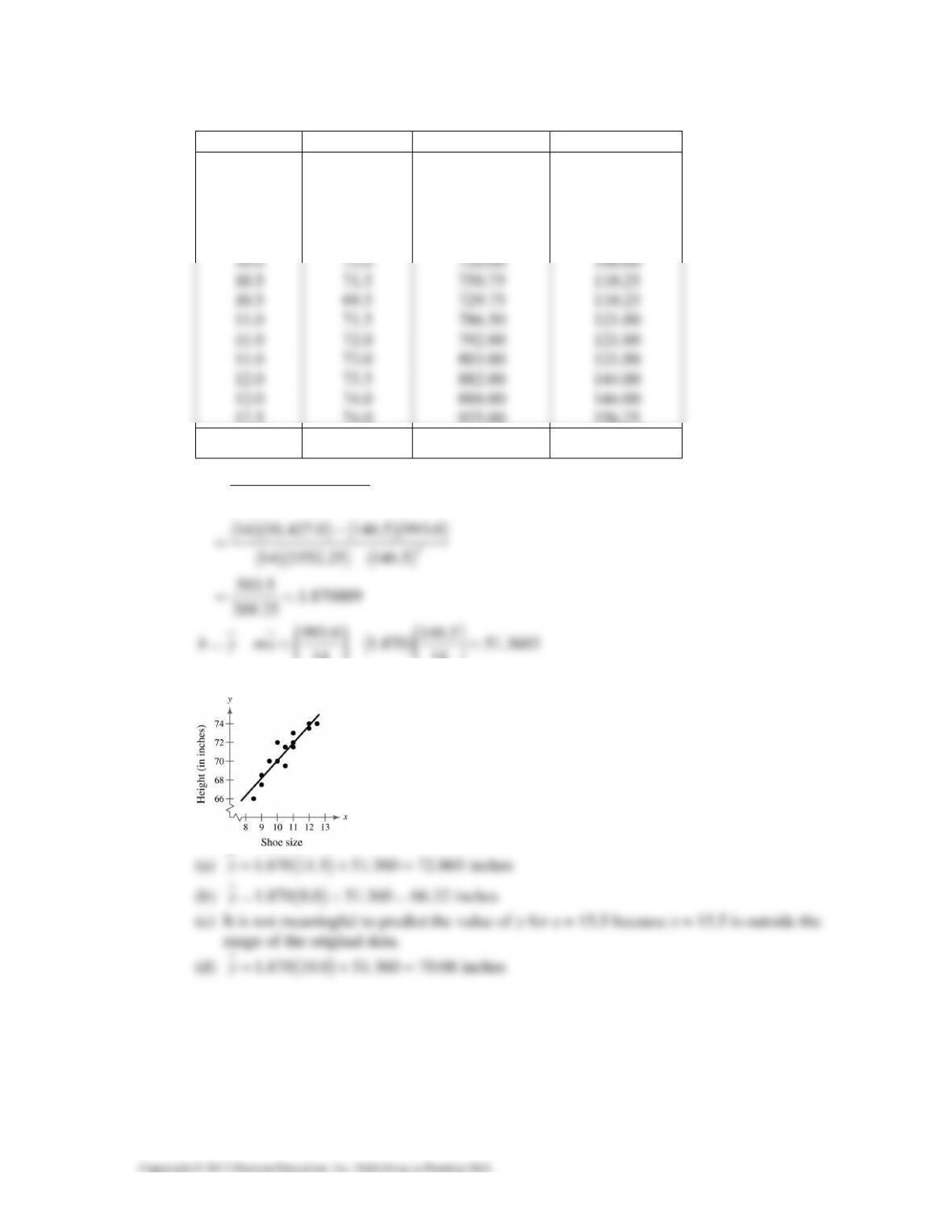
x y xy x2
8.5 66.0 561.00 72.25
9.0 68.5 616.50 81.00
9.0 67.5 607.50 81.00
9.5 70.0 665.00 90.25
10.0 70.0 700.00 100.00
12.5 74.0 925.00 156.25
146.5x=
∑993.0y=
∑10,427.0xy =
∑21552.25x=
∑
()()
()
2
2
xxy x y
m
nx x
∑−∑ ∑
=∑−∑
14 14
⎝⎠ ⎝⎠
1.870 51.360yx=+
374 CHAPTER 9 │ CORREALTION AND REGRESSION
24.
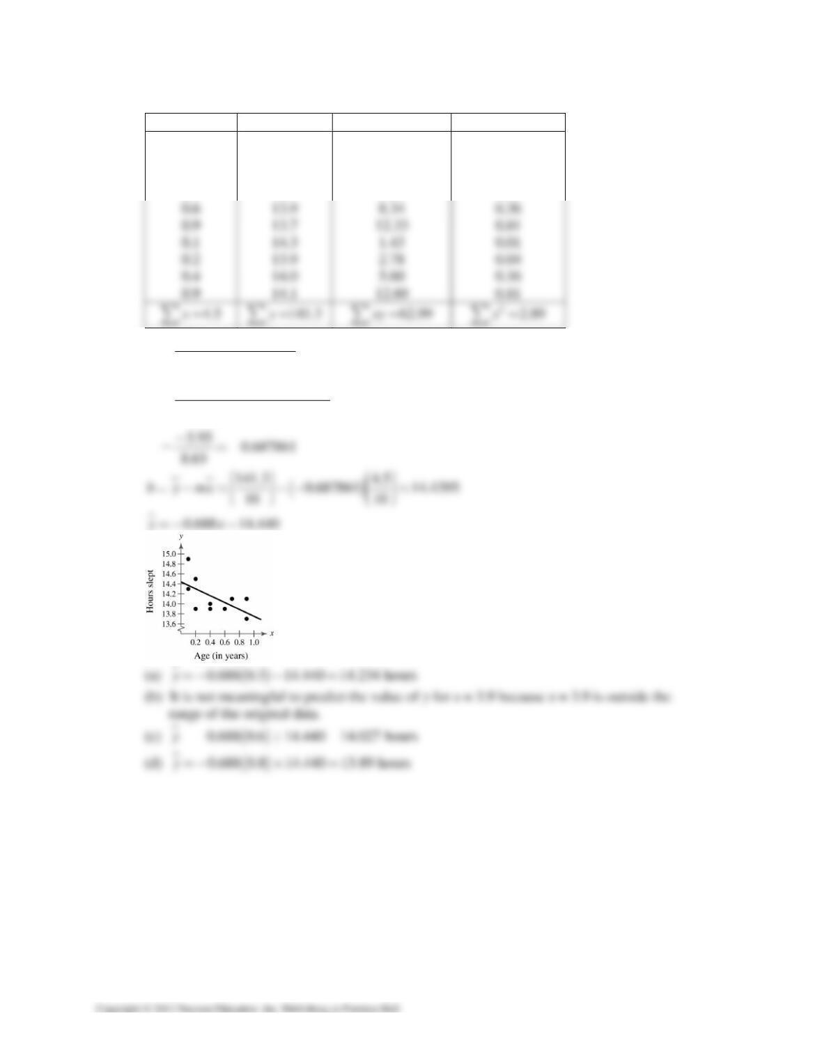
x y xy x2
0.1 14.9 1.49 0.01
0.2 14.5 2.90 0.04
0.4 13.9 5.56 0.16
0.7 14.1 9.87 0.49
()()
()
()( )( )( )
()( )( )
2
2
2
10 62.99 4.5 141.3
10 2.89 4.5
xxy x y
m
nx x
∑−∑ ∑
=∑−∑
−
=−
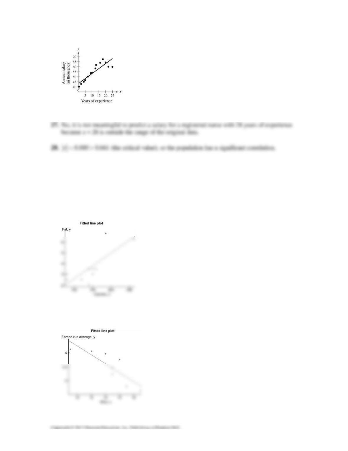
25. Strong positive linear correlation; As the years of experience of registered nurses increase. their
salaries tend to increase.
CHAPTER 9 │ CORRELATION AND REGRESSION 375
26.
43.214 0.9976yx=−
29. Answers will vary. Sample answer: Although it is likely that there is a cause-and-effect
relationship between a registered nurse’s years of experience and salary, the relationship between
variables may also be influenced by other factors, such as work performance, level of education,
or the number of years with an employer.
30a.
0.024 0.181yx=+
b. 0.773r≈
c.
31a.
0.159 5.827yx=− +
b. 0.852r≈−
c.
376 CHAPTER 9 │ CORREALTION AND REGRESSION
32. (a)
1.724 79.733yx=+ (b)
0.453 26.448yx=−
33. (a) (b)
4.297 94.200yx=− +
0.1413 14.763yx=− +
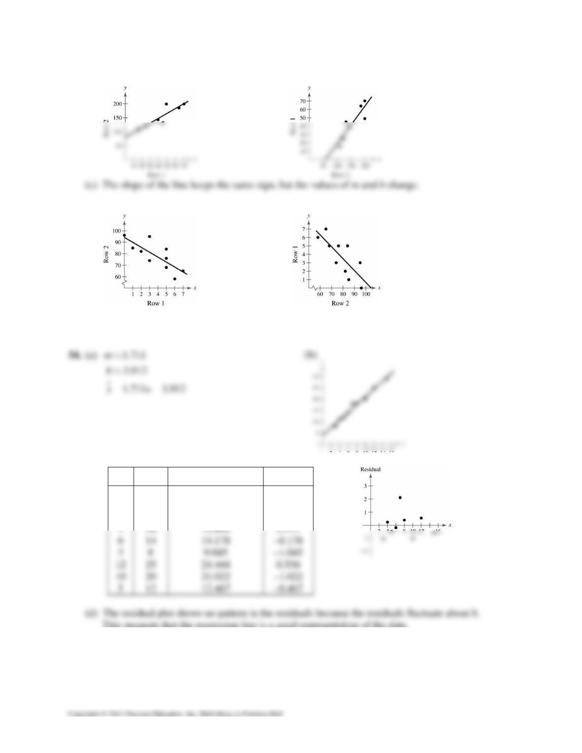
(c) The slope of the line keeps the same sign, but the values of m and b change.
(c)
x y
1.711 3.912yx=+
yy−
8 18 17.600 0.400
4 11 10.756 0.244
15 29 29.577 –0.577
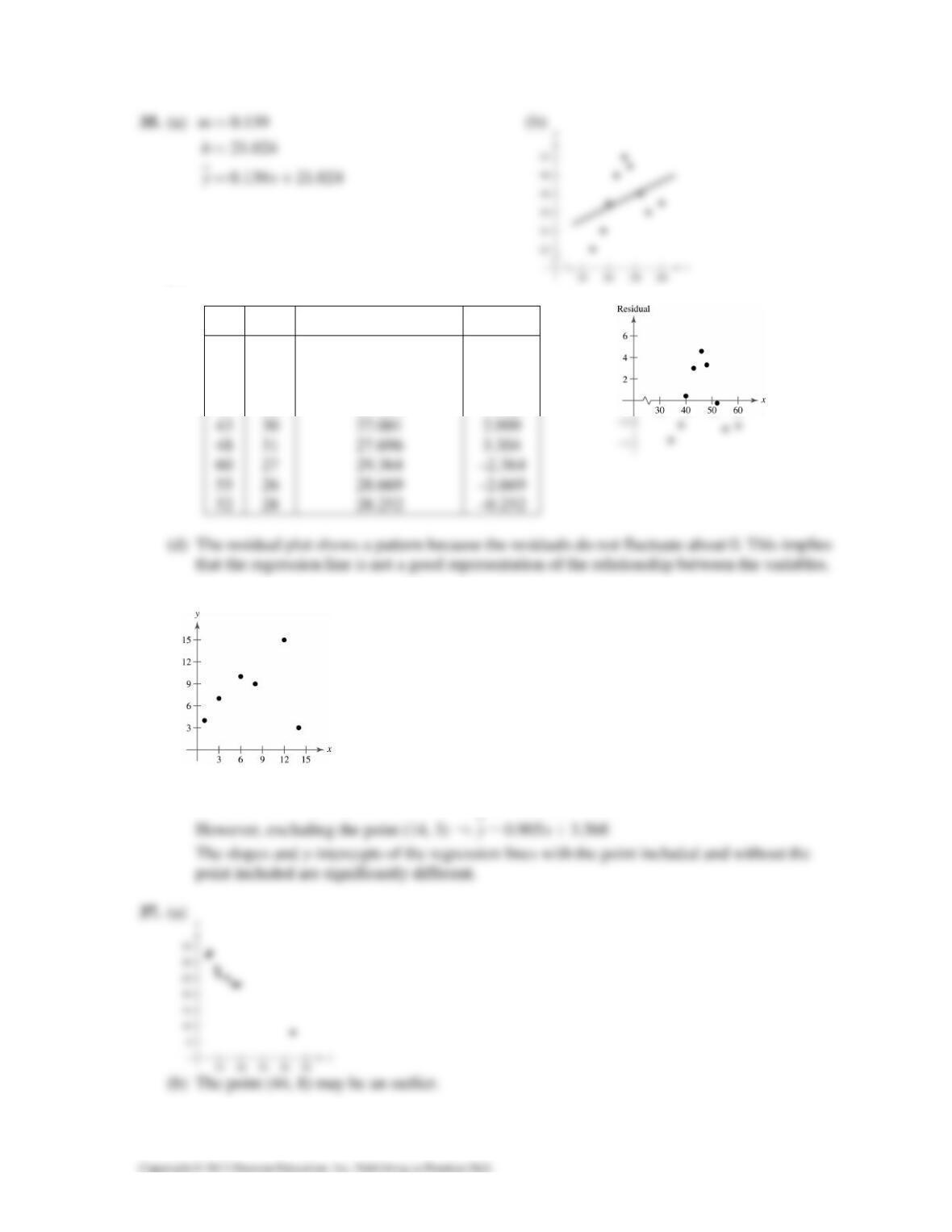
This suggests that the regression line is a good representation of the data.
CHAPTER 9 │ CORRELATION AND REGRESSION 377
(c)
x y
0.139 21.024yx=+
yy−
38 24 26.306 –2.306
34 22 22.750 –3.750
40 27 26.584 0.416
46 32 27.418 4.582
36. (a)
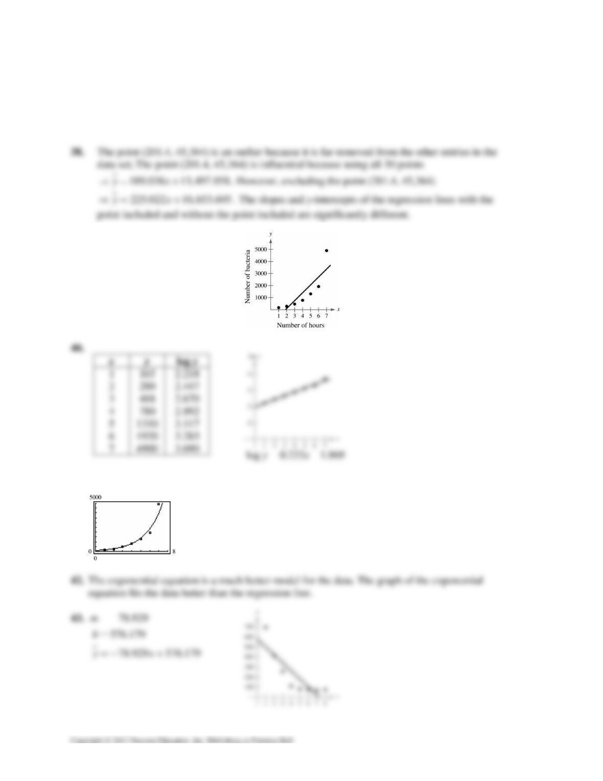
(b) The point (14, 3) may be an outlier.
(c) The point (14, 3) is influential because using all 6 points
0.212 6.445yx⇒= + .
378 CHAPTER 9 │ CORREALTION AND REGRESSION
(c) Excluding the point (44, 8)
0.711 35.263yx⇒=− + . The point (44, 8) is not influential
because using all 8 points
0.607 34.160yx⇒=− + .
The slopes and y–intercepts with the point included and without the point are not
significantly different.
39.
654.536
1214.857
654.536 1214.857
m
b
yx
≈
≈−
=−
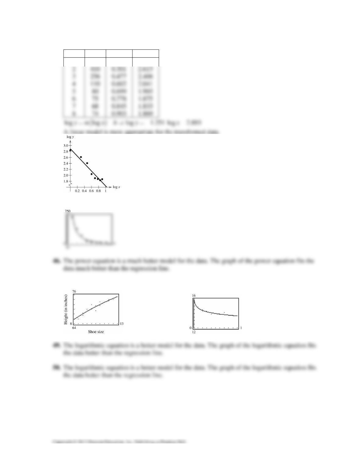
41. Using a technology tool
()
93.028 1.712 x
y⇒= .
CHAPTER 9 │ CORRELATION AND REGRESSION 379
44.
x y log x log y
1 695 0 2.842
45. Using a technology tool 1.251
782.300yx
−
⇒= .
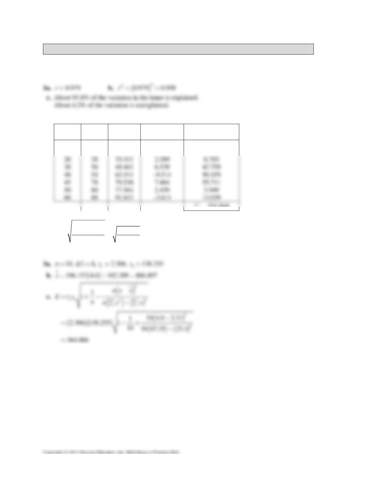
47. ln 25.035 19.599lnyabx x=+ = + 48.
ln 13.8116 0.2966 lnyabx x=+ = −
380 CHAPTER 9 │ CORREALTION AND REGRESSION
9.3 MEASURES OF REGRESSION AND PREDICTION INTERVALS
9.3 Try It Yourself Solutions
2a.
i
x
i
y
i
y
ii
yy−
(
)
2
ii
yy−
15 26 28.386 –2.386 5.693
20 32 35.411 –3.411 11.635
231.948∑=
b. 8n=
c.
l
()
2
231.948 6.218
26
ii
e
yy
sn
∑−
==≈
−
d. The standard error of estimate of the weekly sales for a specific radio ad time is about $621.80.
d.
()
522.809, 1250.985yE+→
e. You can be 95% confident that when the gross domestic product is $4 trillion, the carbon dioxide
emissions will be between 522.809 and 1250.985 million metric tons.
CHAPTER 9 │ CORRELATION AND REGRESSION 381
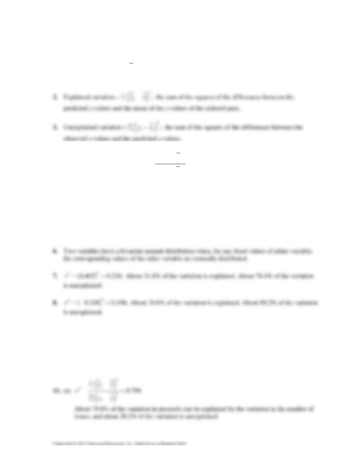
9.3 EXERCISE SOLUTIONS
1. Total variation
()
2;
i
yy=∑ − the sum of the squares of the differences between the y–values of
each ordered pair and the mean of the y–values of the ordered pairs.
4. Coefficient of determination:
()
()
2
2
2
i
i
yy
r
yy
∑−
=
∑−
2
r is the ratio of the explained variation to the total variation and is the percent of variation of y
that is explained by the relationship between x and y. 2
1r− is the percent of variation that is
unexplained.
5. Two variables that have perfect positive or perfect negative linear correlation have a correlation
coefficient of 1 or 1−, respectively. In either case, the coefficient of determination is 1, which
means that 100% of the variation in the response variable is explained by the variation in the
explanatory variable.
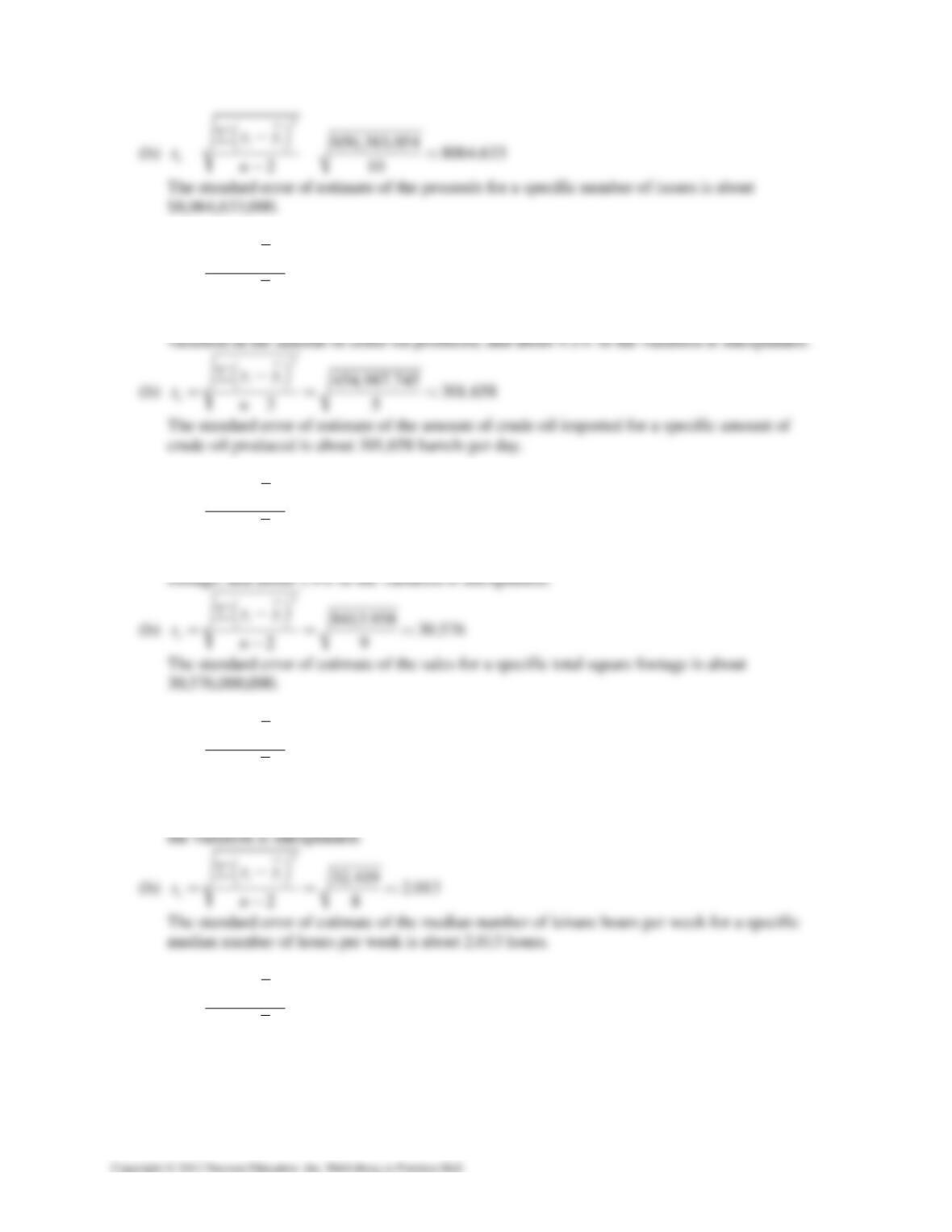
9.
()
2
20.957 0.916;r=− ≈ About 91.6% of the variation is explained. About 8.4% of the variation
is unexplained.
10.
()
2
20.881 0.776;r=≈ About 77.6% of the variation is explained. About 22.4% of the variation
is unexplained.
382 CHAPTER 9 │ CORREALTION AND REGRESSION
12. (a)
()
()
2
2
20.909
i
i
yy
r
yy
∑−
=≈
∑−
About 90.9% of the variation in the amount of crude oil imported can be explained by the
13. (a)
()
()
2
2
20.981
i
i
yy
r
yy
∑−
=≈
∑−
About 98.1% of the variation in sales can be explained by the variation in the total square
14. (a)
()
()
2
2
20.578
i
i
yy
r
yy
∑−
=≈
∑−
About 57.8% of the variation in the median number of leisure hours per week can be
explained by the variation in the median number of work hours per week, and about 42.2% of
15. (a)
()
()
2
2
20.963
i
i
yy
r
yy
∑−
=≈
∑−
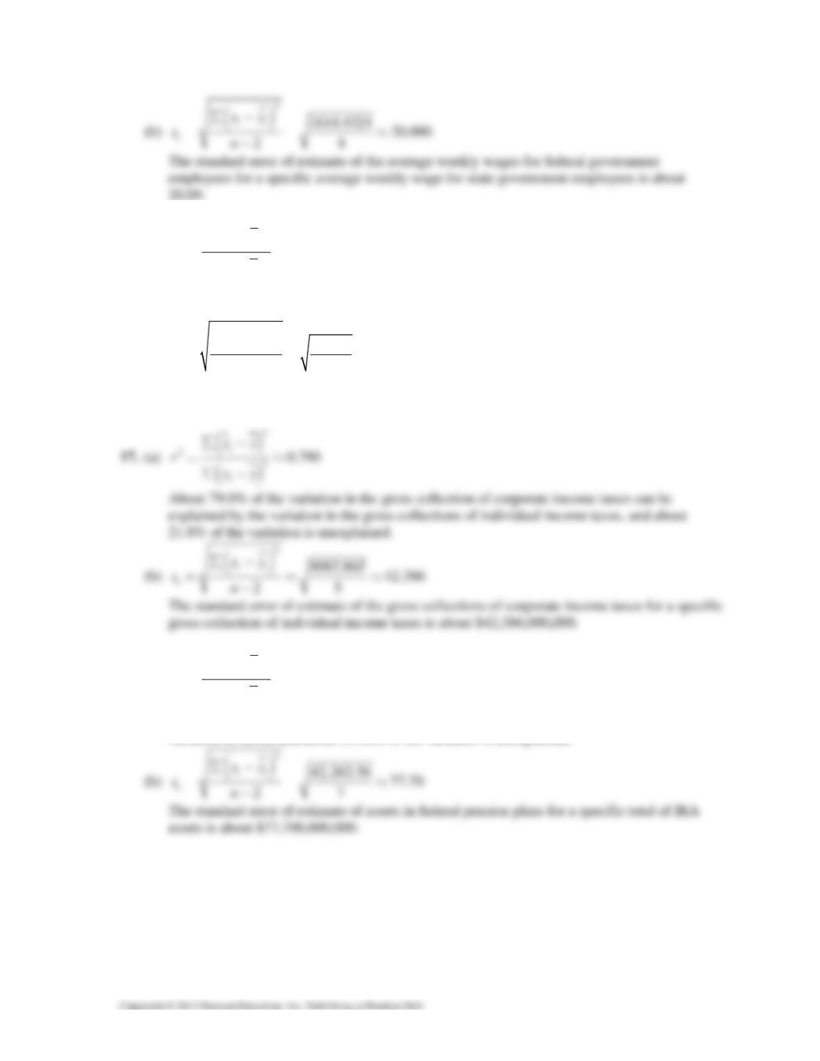
About 96.3% of the variation in wages for federal government employees can be explained
by the variation in wages for state government employees, and about 3.7% of the variation is
unexplained.
CHAPTER 9 │ CORRELATION AND REGRESSION 383
16. (a)
()
()
2
2
20.919
i
i
yy
r
yy
∑−
=≈
∑−
About 91.9% of the variation in the turnout for federal elections can be explained by the
variation in the voting age population, and about 8.1% of the variation is unexplained.
(b)
l
()
2
31.933 2.307
26
ii
e
yy
sn
∑−
==≈
−
The standard error of estimate of the turnout in a federal election for a specific voting age
population is about 2,307,000.
18. (a)
()
()
2
2
20.7704
i
i
yy
r
yy
∑−
=≈
∑−
About 77.04% of the variation in assets in federal pension plans can be explained by the
variation in IRAs, and about 22.96% of the variation is unexplained.
384 CHAPTER 9 │ CORREALTION AND REGRESSION
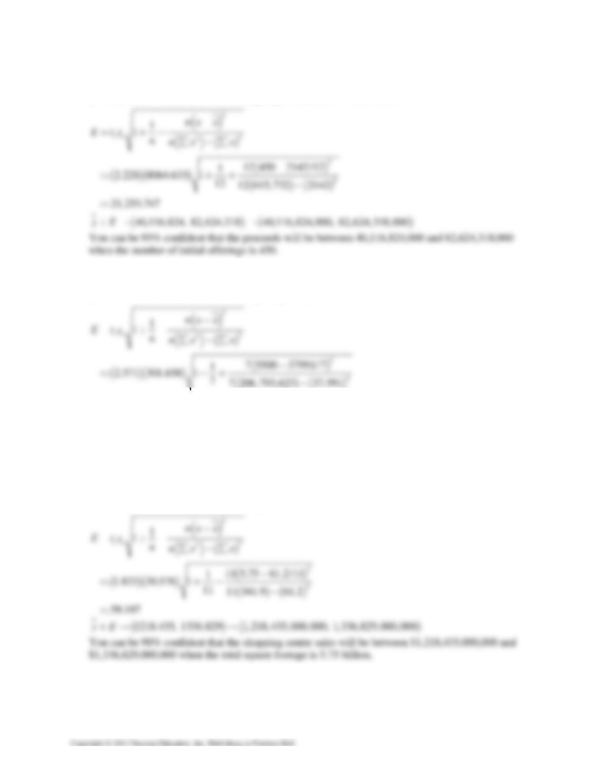
19. 12, d.f. 10, 2.228, 8064.633
ce
nts=== ≈
()
104.982 14,128.671 104.982 450 14,128.671 61,370.571yx=+ = + =
20. 7, d.f. 5, 2.571, 301.658
ce
nts=== ≈
()
2.735 27,657.823 2.735 5500 27,657.823 12,615.323yx=− + =− + =
832.272
≈
()( )
11,783.051, 13, 447.595 11,783,051, 13,447,595yE+→ →
You can be 95% confident that the amount of crude oil imported by the United States will be
between 11,783,051 and 13,447,595 when the amount of crude oil produced by the United States
is 5,500,000 barrels per day.
21. 11, d.f. 9, 1.833, 30.576
ce
nts=== ≈
()
549.448 1881.694 549.448 5.75 1881.694 1277.632yx=−=− −≈
CHAPTER 9 │ CORRELATION AND REGRESSION 385
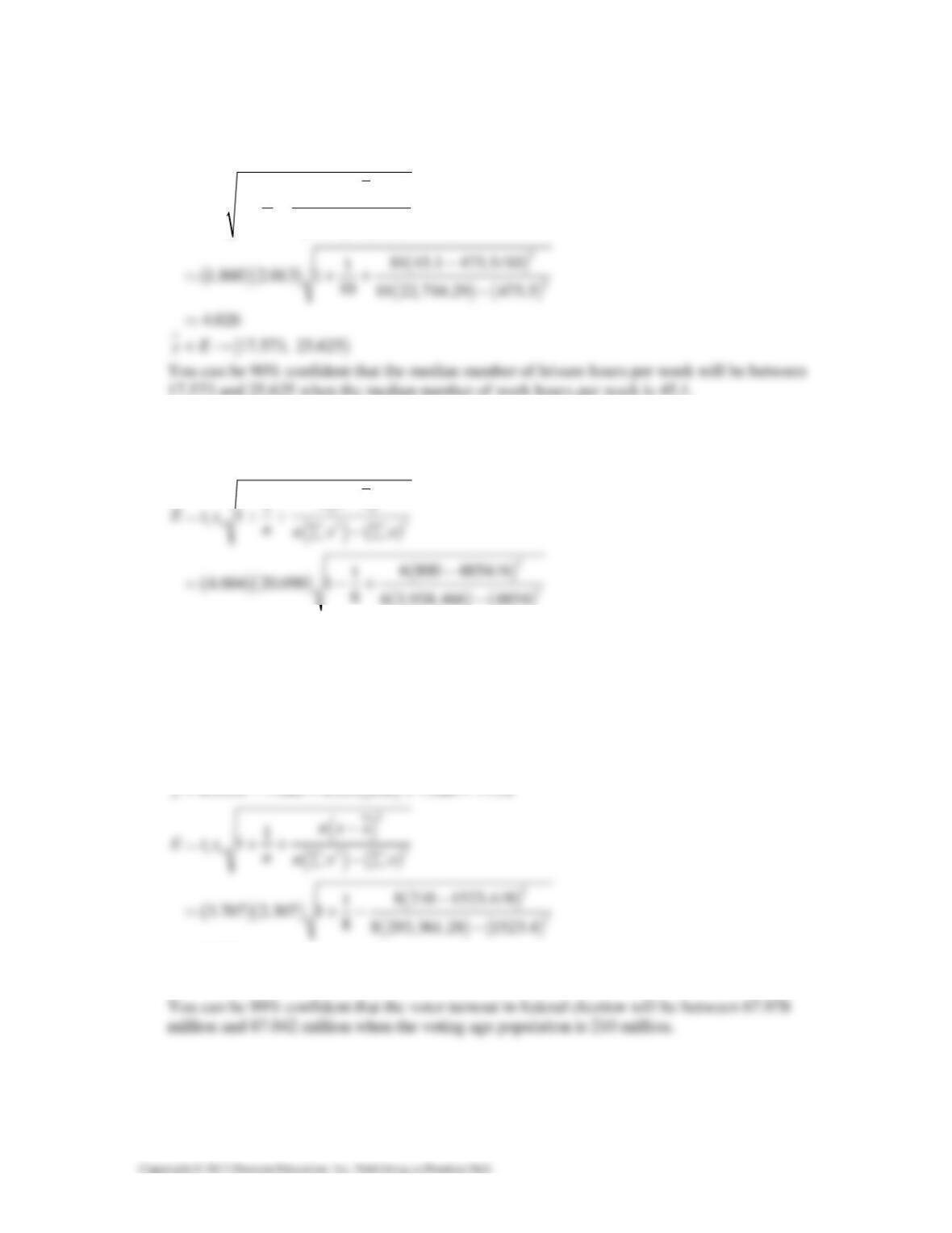
22. 10, d.f. 8, 1.860, 2.013
ce
nts=== ≈
()
0.646 50.734 0.646 45.1 50.734 21.599yx=− + =− + ≈
()
()
()
2
2
2
1
1
ce
nx x
Ets nnx x
−
=++
∑−∑
17.573 and 25.625 when the median number of work hours per week is 45.1.
23. 6, d.f. 4, 4.604, 20.090
ce
nts=== ≈
()
1.900 411.976 1.900 800 411.976 1108.024yx=− = − =
()
2
100.204
nx x
−
≈
()
1007.82, 1208.228yE+→
You can be 99% confident that the average weekly wages of federal government employees will
be between 1007.82 and 1208.23 when the average weekly wage of state government employees
is $800.
24. 8, d.f. 6, 3.707, 2.307
ce
nts
=== ≈
9.532
≈
()
67.978, 87.042yE+→
386 CHAPTER 9 │ CORREALTION AND REGRESSION
25. 7, d.f. 5, 2.571, 42.386
ce
nts=== ≈
()
0.415 186.626 0.415 1250 186.626 332.124yx=− = − ≈
()
2
118.395
nx x
−
≈
()
213.729, 450.519yE+→
You can be 95% confident that the corporate income taxes collected by the U.S. Internal Revenue
Service for a given year will be between $213.729 million and $450.519 million when the U.S.
Internal Revenue Service collects $1.250 million in individual income taxes that year.
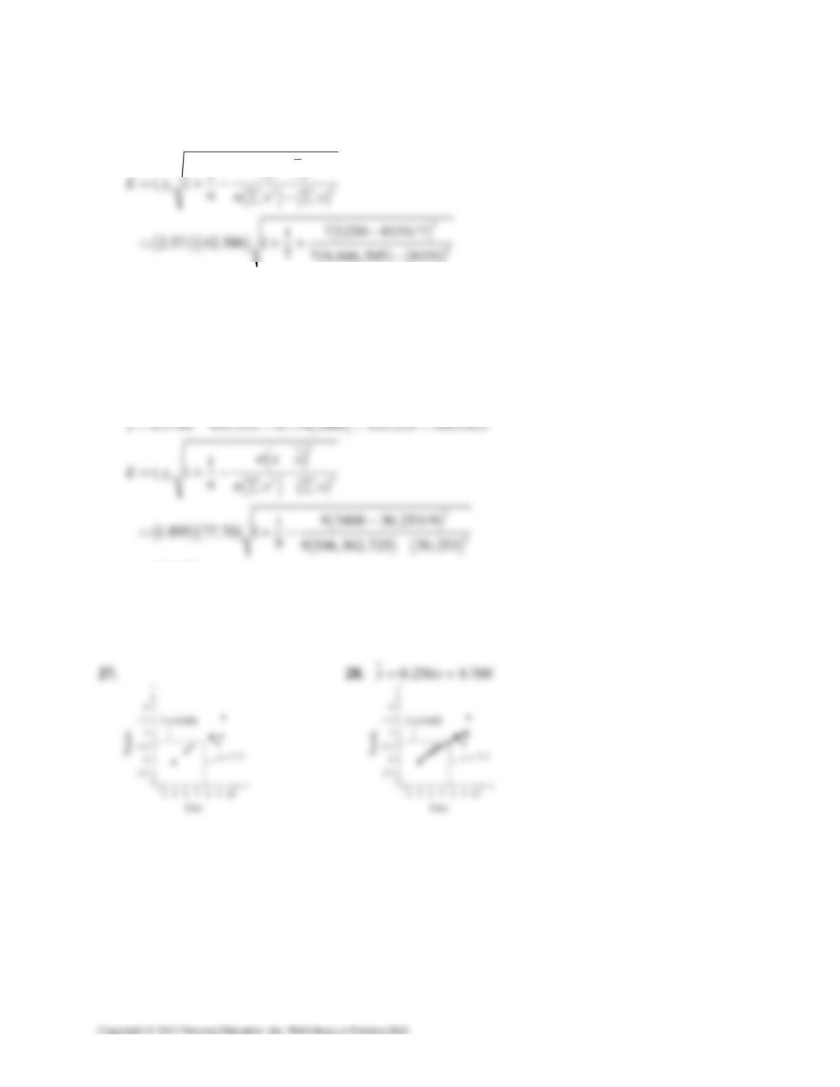
26. 9, d.f. 7, 1.895, 77.70
ce
nts=== ≈
158.057
≈
()
935.368, 1251.482yE+→
You can be 90% confident that the total assets in federal pension plans will be between $935.368
billion and $1251.482 billion when the total assets in IRAs is $3800 billion.