173
CHAPTER 9
BOX-JENKINS (ARIMA) METHODOLOGY
ANSWERS TO PROBLEMS AND CASES
2. t Yt
t
Y
et
4. a. Model Autocorrelations Partial Autocorrelations
5. a. MA(2)
174
b. Q = 44.3 df
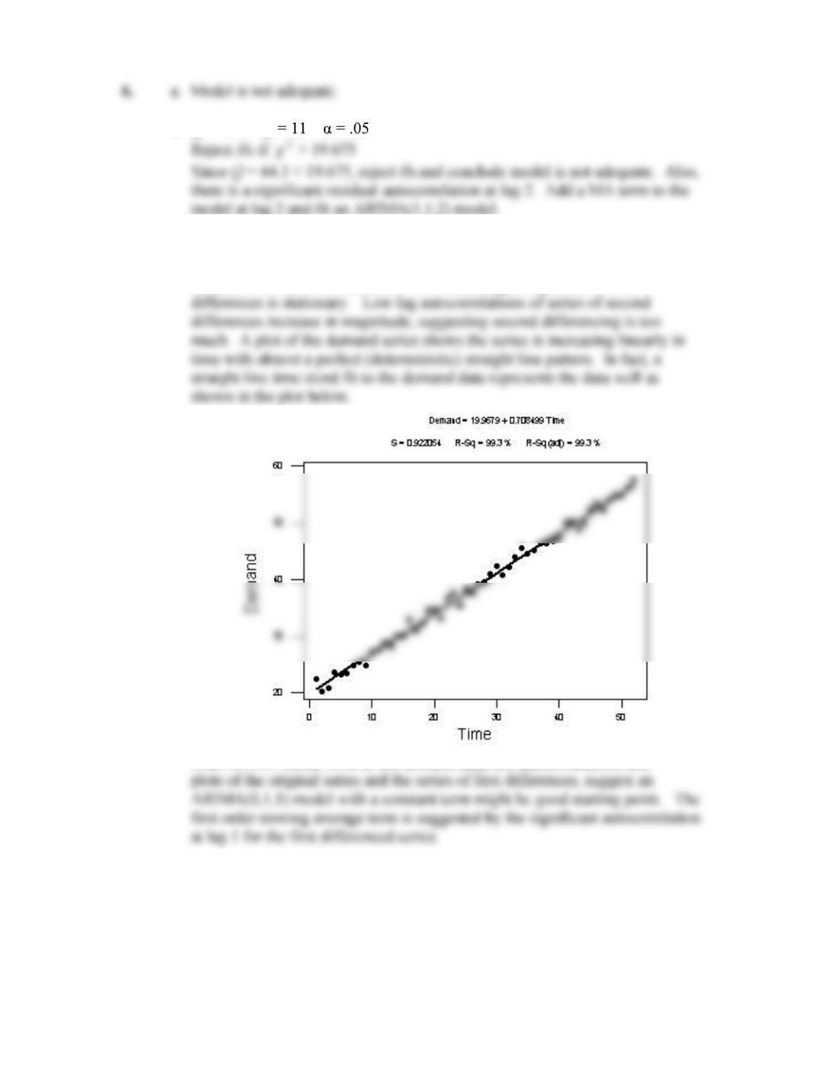
7. a. Autocorrelations of original series fail to die out, suggesting that demand is
non-stationary. Autocorrelations for first differences of demand, do die
out (cut off relative to standard error limits) suggesting series of first
If an ARIMA model is fit to the demand data, the autocorrelations and
b. The Minitab output from fitting an ARIMA(0,1,1) model with a constant is
shown below.
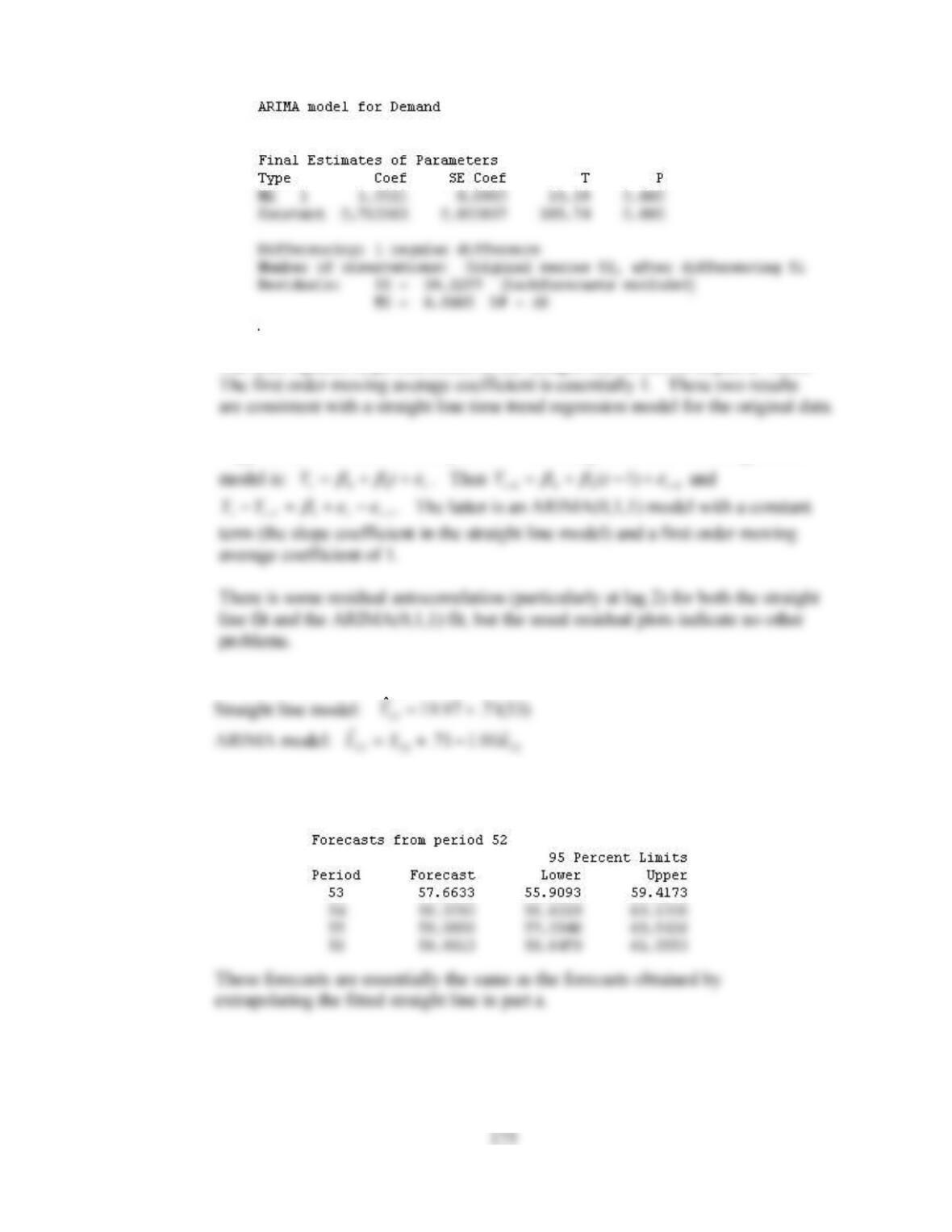
The least squares estimate of the constant term, .7127, is virtually the same as
The least squares slope coefficient in the straight line fit shown in part a. Also,
Suppose
t
Y
is demand in time period t. The straight line time trend regression
c. Prediction equations for period 53.
d. The forecasts for the next four periods from forecast origin t = 52 for the
ARIMA model follow.
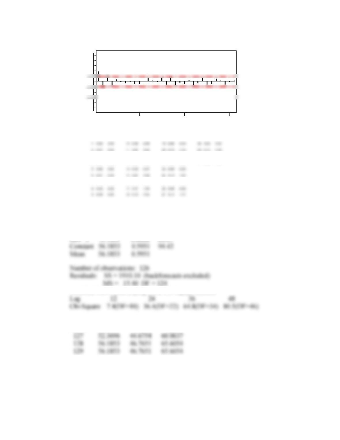
8. Since the autocorrelation coefficients drop off after one time lag and the partial
autocorrelation coefficients trail off, an MA(1) model should be adequate. The best
model is
The forecast for period 127 is
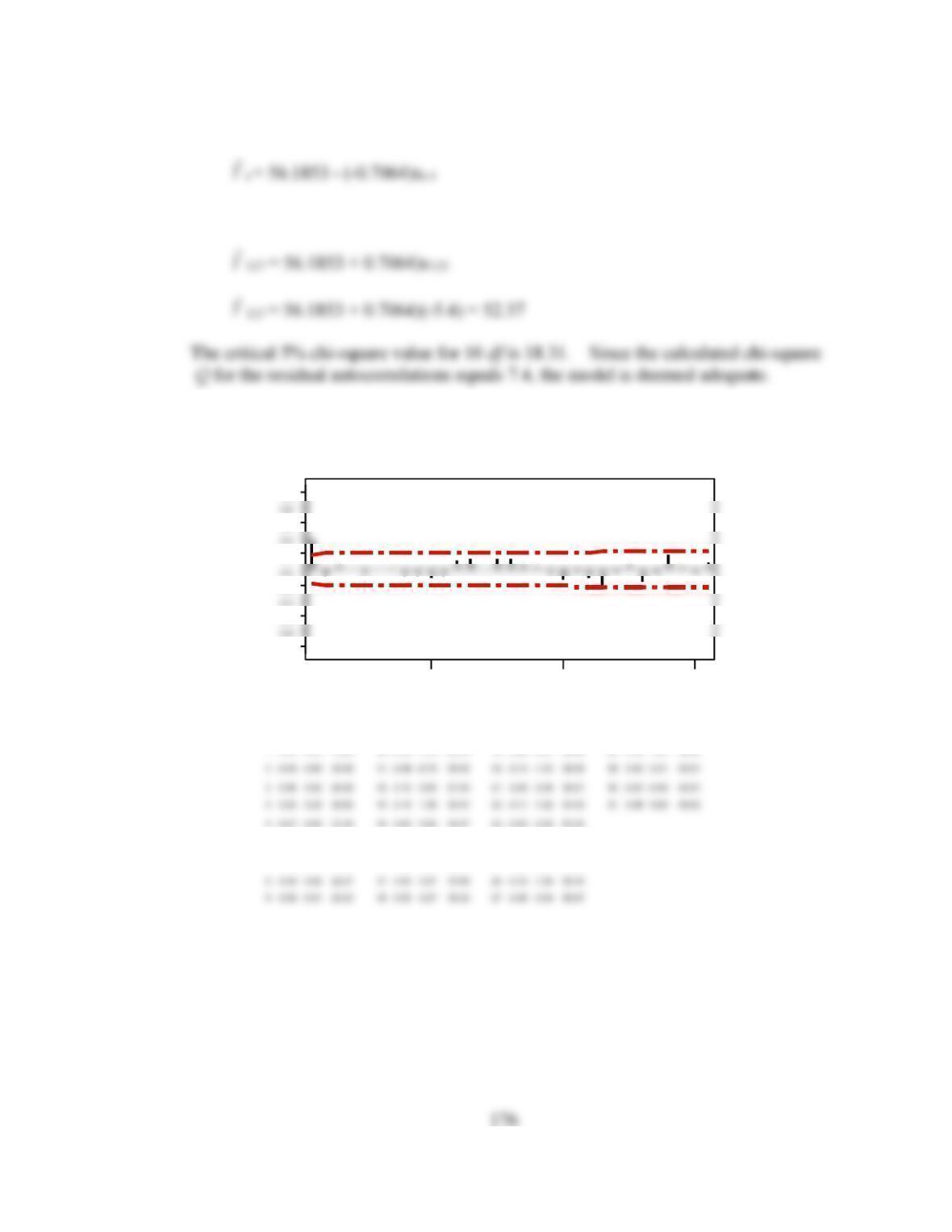
The autocorrelation and partial autocorrelation plots for the original series follow.
302010
1.0
0.6
0.2
-0.2
-0.6
-1.0
LBQTCorrLagLBQTCorrLagLBQTCorrLagLBQTCorrLag
62.90
52.05
51.49
36.49
35.49
32.95
25.16
21.31
21.29
19.20
1.60
0.50
-0.26
-0.51
1.21
1.21
-1.13
-0.12
0.18
4.33
0.19
0.06
-0.03
-0.06
0.13
0.13
-0.12
-0.01
0.02
0.39
28
25
24
19
16
15
10
7
6
1
Autocorrelation Function for Yt
177
302010
1.0
0.8
0.6
0.4
0.0
-0.4
-0.8
-1.0
TPACLagTPACLagTPACLagTPACLag
0.45
-0.05
0.53
0.39
-1.14
0.08
-2.30
0.61
-1.18
0.50
1.41
-0.65
-2.25
2.95
0.04
-0.00
-0.10
-0.20
0.05
-0.11
0.04
0.13
-0.06
-0.20
0.26
31
30
25
22
21
16
13
12
7
4
3
Partial Autocorrelation Function for Yt
ARIMA model for Yt
Final Estimates of Parameters
Type Coef StDev T
MA 1 -0.7064 0.0638 -11.07
Modified Box-Pierce (Ljung-Box) Chi-Square statistic
95 Percent Limits
Period Forecast Lower Upper
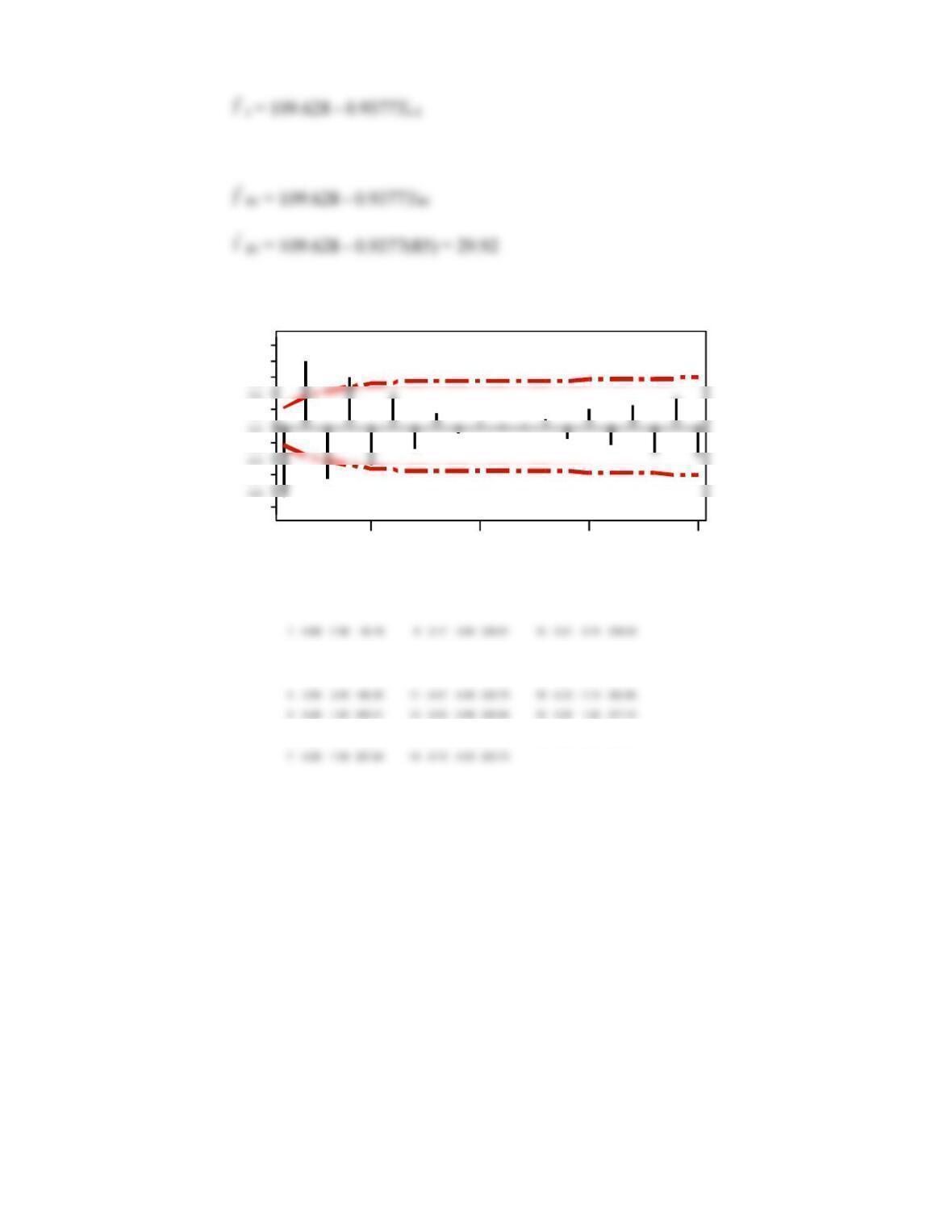
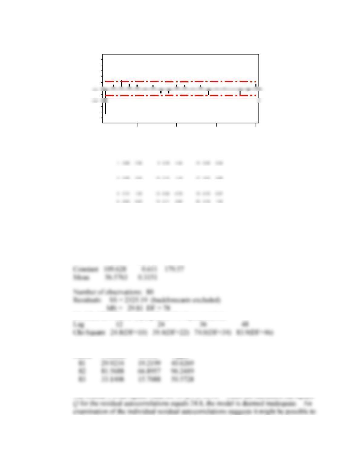
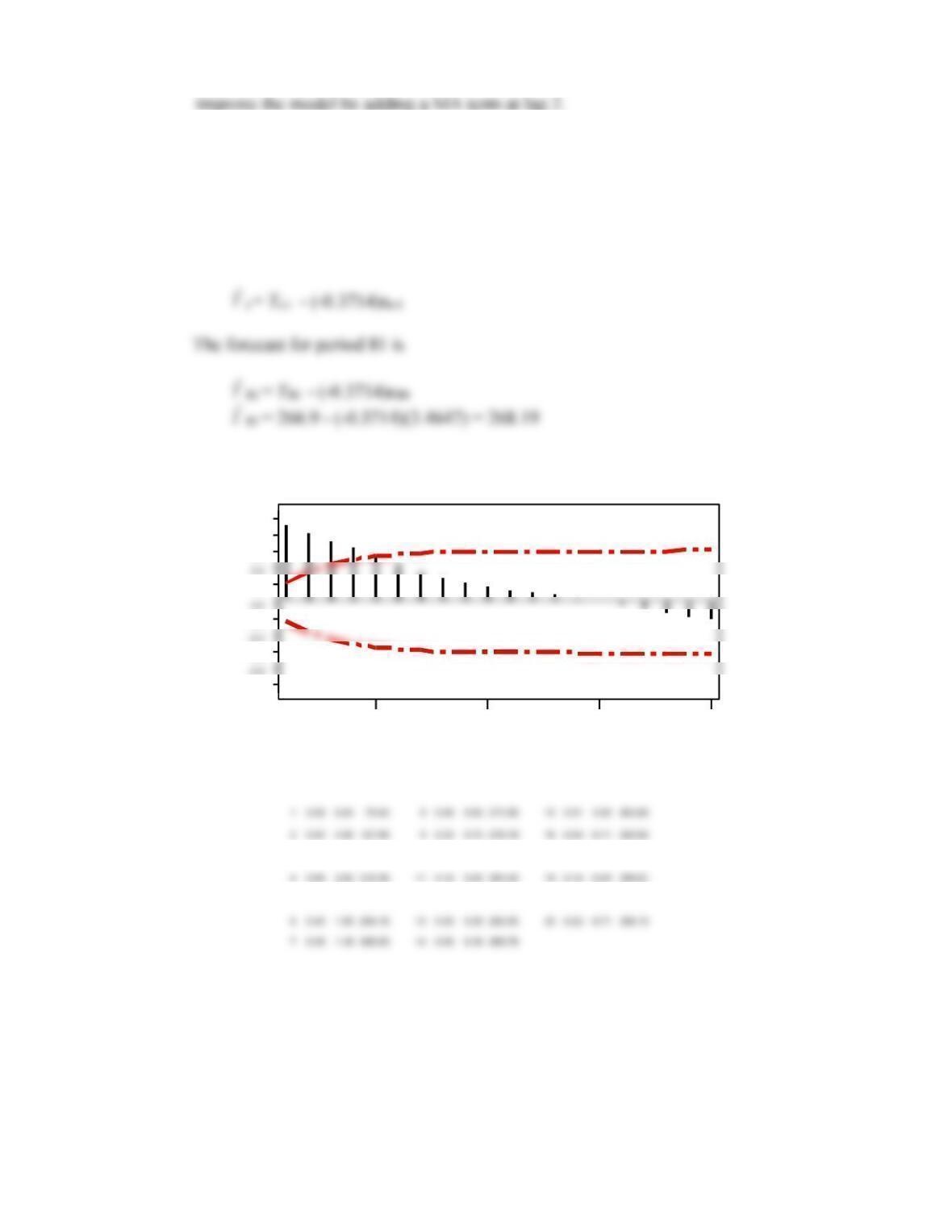
9. Since the autocorrelation coefficients trail off and the partial autocorrelation
coefficients cut off after one time lag, an AR(1) model should be adequate.
The best model is
178
The forecast for period 81 is
2015105
1.0
0.8
0.6
0.2
-0.2
-0.6
-1.0
LBQTCorrLagLBQTCorrLagLBQTCorrLag
293.47
277.15
262.96
230.84
230.79
251.34
244.21
238.24
229.81
233.73
231.46
230.78
230.51
220.35
155.90
118.31
-1.28
0.90
-0.84
0.28
0.19
-0.31
1.47
-3.03
4.50
-0.39
0.26
-0.24
0.08
0.05
-0.09
0.40
-0.66
0.80
20
17
16
13
10
9
6
3
2
Autocorrelation Function for Yt
179
2015105
1.0
0.8
0.6
0.4
0.2
-0.2
-0.6
-0.8
-1.0
TPACLagTPACLagTPACLag
-2.32
0.28
-1.95
1.01
-1.44
1.10
1.43
1.16
-0.26
0.03
-0.22
0.11
-0.16
0.12
0.16
0.13
18
16
14
11
9
7
4
2
Partial Autocorrelation Function for Yt
ARIMA model for Yt
Final Estimates of Parameters
Type Coef StDev T
AR 1 -0.9377 0.0489 -19.17
Modified Box-Pierce (Ljung-Box) Chi-Square statistic
95 Percent Limits
Period Forecast Lower Upper
180
10. As can be seen below, the autocorrelations for the original series are slow to die out. This
behavior indicates the series may be non-stationary. The autocorrelations for the
differenced data cut off after lag 1 and the partial autocorrelations die out. This suggests
an ARIMA(0,1,1) model. When this model is fit (see the computer output below), there
are no significant residual autocorrelations and the residual plots look good. The
forecasting equation from the fitted model is
2015105
1.0
0.8
0.6
0.2
-0.2
-0.6
-1.0
LBQTCorrLagLBQTCorrLagLBQTCorrLag
290.72
284.72
282.83
279.67
236.52
174.43
-0.62
-0.28
0.38
0.58
2.00
3.28
-0.19
-0.09
0.12
0.18
0.55
0.74
19
17
12
10
5
3
Autocorrelation Function for Yt
ARIMA model for Yt
Final Estimates of Parameters
Type Coef StDev T
Differencing: 1 regular difference
Number of observations: Original series 80, after differencing 79
Modified Box-Pierce (Ljung-Box) Chi-Square statistic
95 Percent Limits
Period Forecast Lower Upper
11. The slow decline in the early, non-seasonal lags indicates the need for regular
differencing.
22122
1.0
0.8
0.6
0.2
-0.2
-0.6
-1.0
LBQT
Corr
LagLBQTCorrLagLBQT
Corr
Lag
LBQT
Corr
Lag
634.13
610.88
525.09
337.18
88.66
1.85
4.34
0.26
0.50
602.29
595.80
487.93
279.06
1.28
2.39
0.41
586.38
468.47
242.61
1.56
2.41
0.49
574.97
559.60
387.14
168.41
1.74
3.23
0.50
546.38
506.38
441.38
359.38
309.89
210.04
128.66
49.43
1.18
0.64
1.03
1.26
1.22
2.34
1.61
2.07
2.98
3.69
6.92
0.42
0.23
0.35
0.42
0.40
0.70
0.45
0.54
0.63
0.63
0.71
24
22
19
17
15
12
10
8
5
3
1
Autocorrelation Function for Yt
182
25155
1.0
0.8
0.6
0.2
-0.2
-0.6
-0.8
-1.0
LBQTCorrLagLBQTCorrLagLBQTCorrLagLBQTCorrLag
158.67
156.06
118.13
109.87
91.10
90.84
26.06
25.78
15.08
12.19
107.79
107.52
107.44
89.05
85.04
23.41
18.65
105.13
98.33
90.72
38.14
29.20
25.76
15.16
15.09
-0.71
2.98
0.26
-1.38
1.47
-0.73
-2.22
-1.35
1.21
-0.23
0.07
-0.14
0.54
0.05
-0.24
0.25
-0.12
-0.29
-0.17
0.15
-0.03
0.01
25
24
21
18
17
14
11
10
7
4
3
The peaks at lags 12 and 24 are apparent. The seasonal autocorrelation
183
25155
1.0
0.8
0.6
0.2
-0.2
-0.6
-0.8
-1.0
LBQTCorrLagLBQTCorrLagLBQTCorrLagLBQTCorrLag
70.65
0.20
0.03
70.51
70.48
70.43
0.12
0.02
70.36
67.63
61.38
23.89
22.38
20.61
0.10
-0.28
1.22
1.45
-0.50
0.67
0.30
0.02
-0.05
0.21
0.24
-0.07
0.09
0.04
24
20
17
13
10
6
3
25155
1.0
0.8
0.6
0.4
0.2
-0.2
-0.6
-0.8
-1.0
TPACLagTPACLagTPACLagTPACLag
0.34
1.36
-0.38
-0.81
-0.37
-0.07
-0.66
-3.14
-4.44
0.15
-0.04
-0.09
-0.04
-0.01
-0.07
-0.34
-0.49
23
22
16
15
9
8
2
1
Partial Autocorrelation Function for Seasonal
Concentrating on the non-seasonal lags, the autocorrelation coefficients drop off
after one time lag and the partial autocorrelation coefficients trail off, so a regular
Final Estimates of Parameters
Type Coef StDev T
Differencing: 1 regular, 1 seasonal of order 12
Number of observations: Original series 96, after differencing 83
Modified Box-Pierce (Ljung-Box) Chi-Square statistic
95 Percent Limits
Period Forecast Lower Upper
100 178792 160785 196798
101 188706 170227 207185
b. The autocorrelation coefficient plot below indicates that the data are
185
A
1272
1.0
0.8
0.6
0.2
-0.2
-0.4
-0.6
-1.0
LBQTCorrLagLBQTCorrLag
147.91
135.27
147.60
147.18
116.50
146.21
145.12
74.38
143.50
140.30
128.06
99.23
42.05
0.23
0.37
0.66
1.40
2.48
6.30
0.08
0.13
0.22
0.44
0.66
0.87
12
10
8
5
3
1
1272
1.0
0.8
0.6
0.4
0.0
-0.4
-0.6
-0.8
-1.0
LBQTCorrLagLBQTCorrLag
16.74
6.44
6.19
5.42
16.45
16.44
5.34
0.06
13.24
6.86
4.77
0.30
5.40
5.17
-0.05
-2.01
0.20
0.56
-0.01
-0.31
0.03
0.08
11
9
4
2
Autocorrelation Function for Diff.
186
12
7
2
1.0
0.8
0.6
0.4
0.2
-0.2
-0.6
-0.8
-1.0
T
PAC
Lag
T
PAC
Lag
0.72
-2.11
-0.43
0.04
-0.03
2.12
0.10
-0.30
-0.06
0.01
-0.00
0.30
11
9
8
4
2
1
c. There is not much going on in either the autocorrelations or partial autocorrelations
for the differenced series. Could make a case for a first order AR term in a model
ARIMA model for IBM
Final Estimates of Parameters
AR 1 0.3780 0.1496 2.53 .015
Differencing: 1 regular difference
Number of observations: Original series 52, after differencing 51
Modified Box-Pierce (Ljung-Box) Chi-Square statistic
95 Percent Limits
Period Forecast Lower Upper
187
d. The residual plots look good and there are no significant residual autocorrelations.
There is no reason to doubt the adequacy of the model.
e.
Y
t = Yt-1 + .378(Yt – Yt-1)
13. One question that might arise is should the student use the first 145 observations or
all 150 observations. With this many observations, it will not make much difference.
188
It appears that the autocorrelations for the differenced data cut off after lag one
and that the partial autocorrelations die out. This suggests a regular MA term in a model
The computer output for the fitted model is given below.
Final Estimates of Parameters
Type Coef SE Coef T P
Modified Box-Pierce (Ljung-Box) Chi-Square statistic
Lag 12 24 36 48
95% Limits
Period Forecast Lower Upper Actual
147 133.814 128.637 138.991 139.2
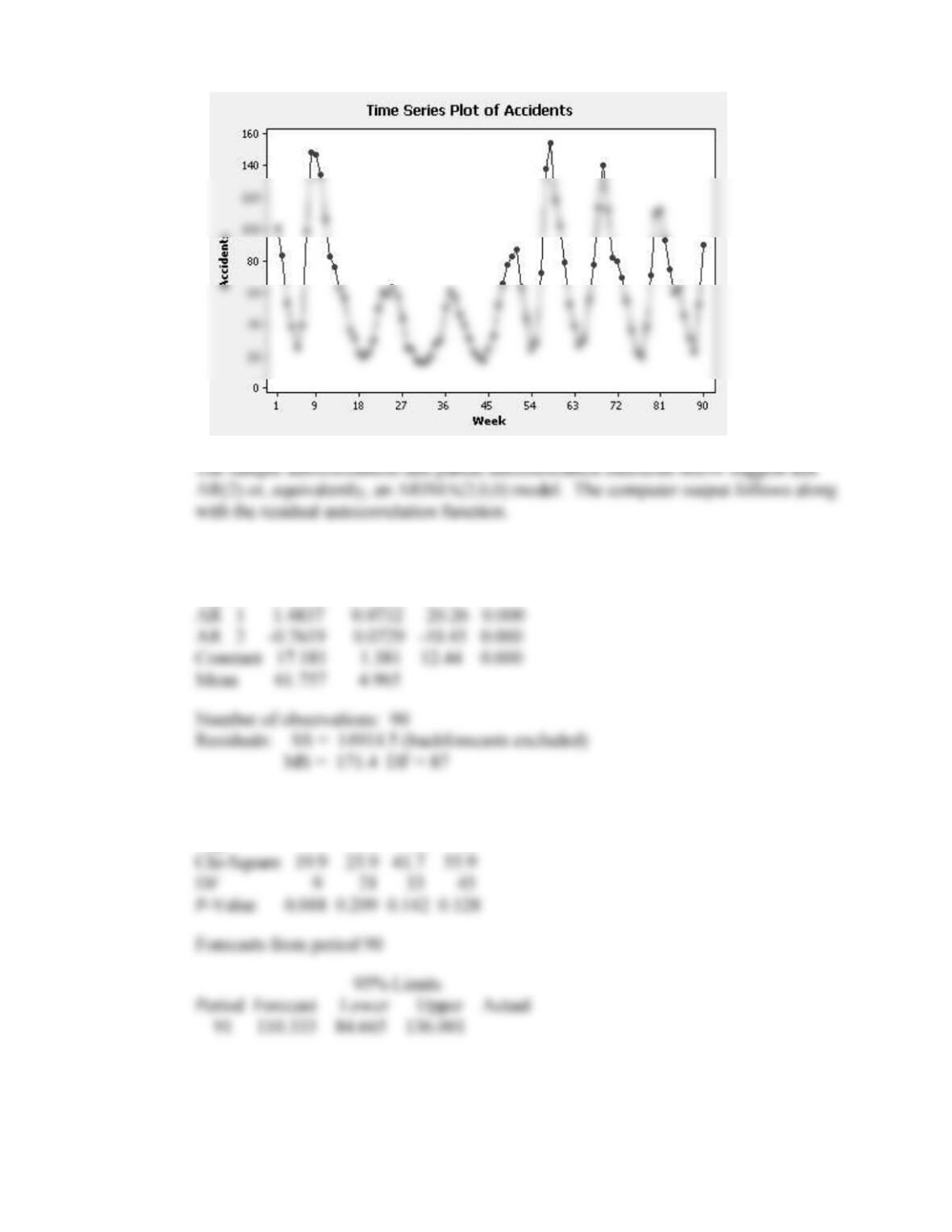
14. The time series plot follows.
190
Final Estimates of Parameters
Type Coef SE Coef T P
Modified Box-Pierce (Ljung-Box) Chi-Square statistic
Lag 12 24 36 48
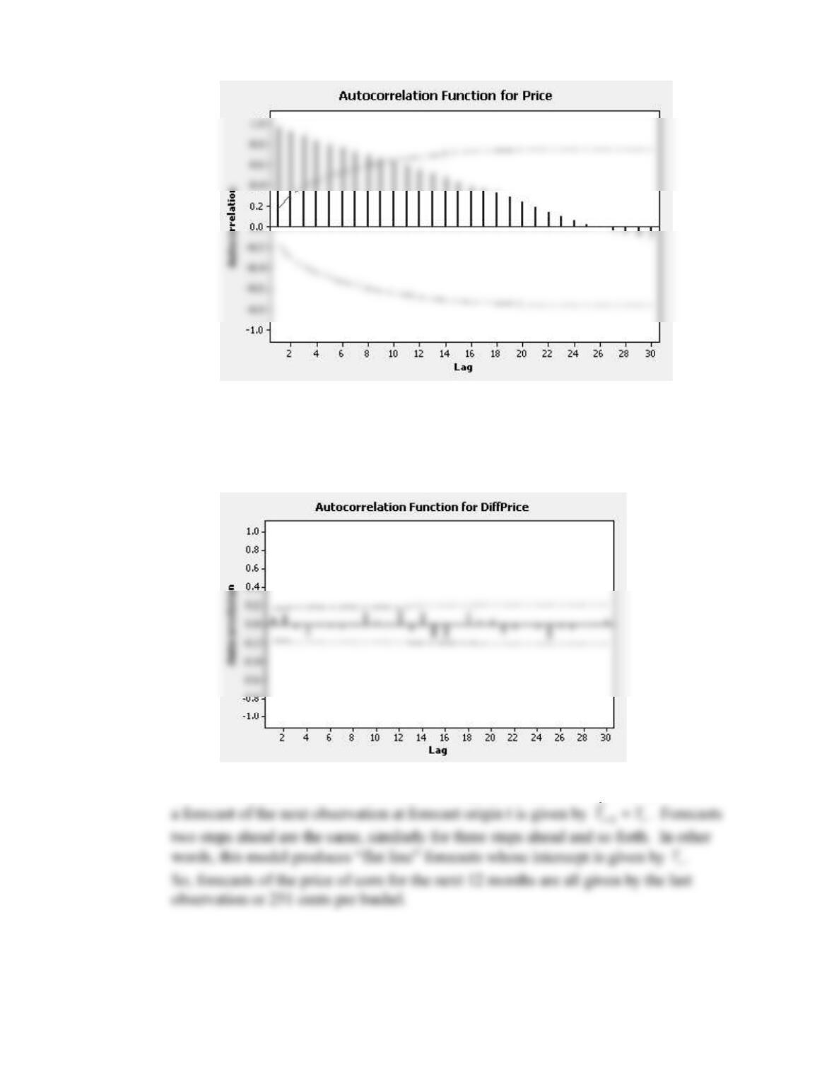
15. The time series plot that follows suggests the Price series is non-stationary. This
is corroborated by the autocorrelations which are slow to die out. The differenced
series should be investigated.
192
The autocorrelation function for the differenced data below suggests the
differenced series is random. The partial autocorrelation function for the
differenced data has a similar appearance.
An ARIMA(0,1,0) model is identified for the price of corn. For this model
16. The variation in the Cavanaugh sales series increases with the level, so a log