CHAPTER 8 – 1
CHAPTER 9
MAKING CAPITAL INVESTMENT
DECISIONS
Answers to Concepts Review and Critical Thinking Questions
1. In this context, an opportunity cost refers to the value of an asset or other input that will be used in a
project. The relevant cost is what the asset or input is actually worth today, not, for example, what it
cost to acquire.
3. It’s probably only a mild over-simplification. Current liabilities will all be paid presumably. The cash
portion of current assets will be retrieved. Some receivables won’t be collected, and some inventory
will not be sold, of course. Counterbalancing these losses is the fact that inventory sold above cost
(and not replaced at the end of the project’s life) acts to increase working capital. These effects tend
to offset.
flows.
6. There are two particularly important considerations. The first is erosion. Will the essentialized book
simply displace copies of the existing book that would have otherwise been sold? This is of special
concern given the lower price. The second consideration is competition. Will other publishers step in
and produce such a product? If so, then any erosion is much less relevant. A particular concern to book
publishers (and producers of a variety of other product types) is that the publisher only makes money
from the sale of new books. Thus, it is important to examine whether the new book would displace
sales of used books (good from the publisher’s perspective) or new books (not good). The concern
arises any time that there is an active market for used product.
CHAPTER 8 – 2
8. One company may be able to produce at lower incremental cost or market better. Also, of course, one
of the two may have made a mistake!
9. Porsche would recognize that the outsized profits would dwindle as more products come to market
and competition becomes more intense.
12. The implication is that they will face hard capital rationing.
13. Forecasting risk is the risk that a poor decision is made because of errors in projected cash flows.
The danger is greatest with a new project because the cash flows are usually harder to predict.
Solutions to Questions and Problems
Basic
NOTE: All end-of-chapter problems were solved using a spreadsheet. Many problems require multiple
steps. Due to space and readability constraints, when these intermediate steps are included in this solutions
manual, rounding may appear to have occurred. However, the final answer for each problem is found
without rounding during any step in the problem.
CHAPTER 8 – 3
Increased sales of the motor home line occur because of the new product line introduction; thus:
2,500($77,000) = $192,500,000
3. We need to construct an income statement. The income statement is:
Sales $ 645,000
Variable costs 258,000
Fixed costs 168,000
Depreciation 83,000
EBIT $ 136,000
Taxes@35% 47,600
Net income $ 88,400
4. To find the OCF, we need to complete the income statement as follows:
Sales $ 558,400
Variable costs 346,800
The depreciation tax shield is the depreciation times the tax rate, so:
Depreciation tax shield = Depreciation(TC)
Depreciation tax shield = .35($94,500)
Depreciation tax shield = $33,075
CHAPTER 8 – 4
5. The MACRS depreciation schedule is shown in Table 9.7. The ending book value for any year is the
beginning book value minus the depreciation for the year. Remember, to find the amount of
depreciation for any year, you multiply the purchase price of the asset times the MACRS percentage
for the year. The depreciation schedule for this asset is:
Beginning
Year
Beginning
Book Value
Depreciation
Depreciation
Allowance
Ending
Book Value
1
$715,000.00
14.29%
$102,173.50
$612,826.50
6. The asset has a useful life of 8 years and we want to find the book value of the asset after 5 years. With
straight-line depreciation, the depreciation each year will be:
Annual depreciation = $545,000 / 8
Annual depreciation = $68,125
The asset is sold at a loss to book value, so the depreciation tax shield of the loss is recaptured.
Aftertax salvage value = $95,000 + ($204,375 – 95,000)(.35)
Aftertax salvage value = $133,281.25
To find the taxes on salvage value, remember to use the equation:
5
6
7
CHAPTER 8 – 5
7. To find the book value at the end of four years, we need to find the accumulated depreciation for the
first four years. We could calculate a table as in Problem 5, but an easier way is to add the MACRS
depreciation amounts for each of the first four years and multiply this percentage times the cost of the
asset. We can then subtract this from the asset cost. Doing so, we get:
8. We need to calculate the OCF, so we need an income statement. The lost sales of the current sound
board sold by the company will be a negative since it will lose the sales.
Sales of new
$40,950,000
Lost sales of old
–8,217,000
Variable costs
18,003,150
Fixed costs
Depreciation
EBT
$9,379,850
Tax
Net income
9. Using the tax shield approach to calculating OCF (Remember the approach is irrelevant; the final
answer will be the same no matter which of the four methods you use.), we get:
OCF = (Sales – Costs)(1 – TC) + Depreciation(TC)
OCF = ($2,145,000 – 1,205,000)(1 – .35) + .35($1,950,000 / 3)
OCF = $838,500
CHAPTER 8 – 6
11. The cash outflow at the beginning of the project will increase because of the spending on NWC. At
the end of the project, the company will recover the NWC, so it will be a cash inflow. The sale of the
equipment will result in a cash inflow, but we must also account for the taxes that will be paid on this
sale. So, the cash flows for each year of the project will be:
Year
Cash Flow
0
–$2,100,000
= –$1,950,000 – 150,000
1
838,500
0
= –$1,950,000 – 150,000
1
= ($940,000)(.65) + .35($649,935)
2
= ($940,000)(.65) + .35($866,775)
3
= ($940,000)(.65) + .35($288,795) + 164,323 + 150,000
12. First, we will calculate the annual depreciation for the equipment necessary for the project. The
depreciation amount each year will be:
Year 1 depreciation = $1,950,000(.3333) = $649,935
Year 2 depreciation = $1,950,000(.4445) = $866,775
Year 3 depreciation = $1,950,000(.1481) = $288,795
So, the book value of the equipment at the end of three years, which will be the initial investment
minus the accumulated depreciation, is:
2
3
1,102,250
= $838,500 + 150,000 + 175,000 + (0 – 175,000)(.35)
CHAPTER 8 – 7
Remember to include the NWC cost in Year 0, and the recovery of the NWC at the end of the project.
The NPV of the project with these assumptions is:
13. First, we will calculate the annual depreciation of the new equipment. It will be:
Annual depreciation = $655,000 / 5
Annual depreciation = $131,000
Now, we calculate the aftertax salvage value. The aftertax salvage value is the market price minus (or
plus) the taxes on the sale of the equipment, so:
Aftertax salvage value = MV + (0 – MV)TC
Aftertax salvage value = MV(1 – TC)
We will use this equation to find the aftertax salvage value since we know the book value is zero. So,
the aftertax salvage value is:
14. First, we will calculate the annual depreciation of the new equipment. It will be:
Annual depreciation charge = $410,000 / 5
Annual depreciation charge = $82,000
The aftertax salvage value of the equipment is:
Aftertax salvage value = $30,000(1 – .35)
Aftertax salvage value = $19,500
CHAPTER 8 – 8
15. To evaluate the project with a $145,000 cost savings, we need the OCF to compute the NPV. Using
the tax shield approach, the OCF is:
OCF = $145,000(1 – .35) + .35($82,000)
OCF = $122,950
NPV = –$410,000 + 35,000 + $122,950(PVIFA10%,5) + [($19,500 – 35,000) / (1.10)5]
NPV = $81,452.95
16. The base-case, best-case, and worst-case values are shown below. Remember that in the best-case,
sales and price increase, while costs decrease. In the worst case, sales and price decrease, and costs
increase.
Scenario
Unit Sales
Unit Price
Unit Variable Cost
Fixed Costs
Base case
55,000
$960
$350
$3,600,000
Best case
63,250
$298
$3,060,000
Worst case
46,750
$816
$403
$4,140,000
CHAPTER 8 – 9
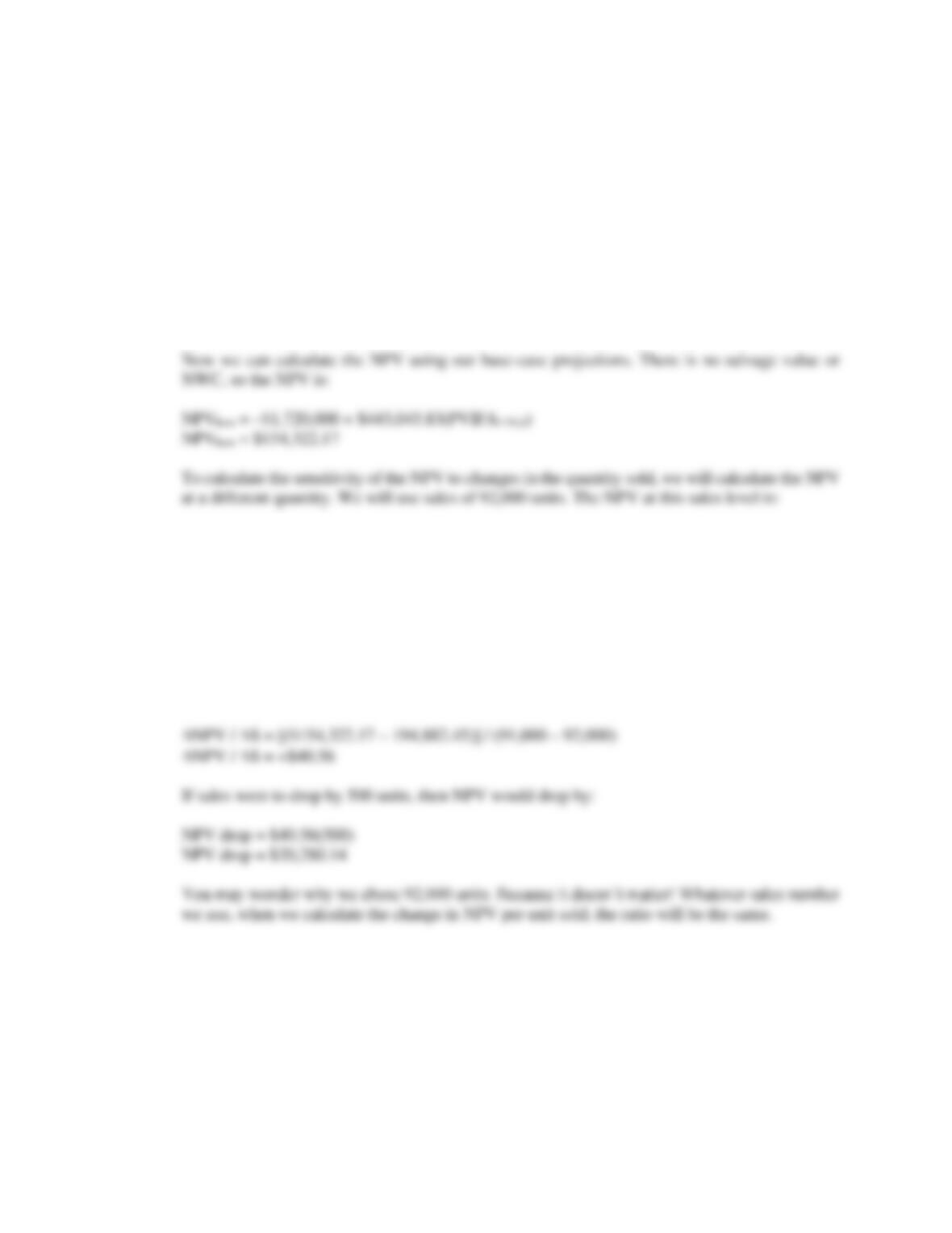
17. An estimate for the impact of changes in price on the profitability of the project can be found from the
sensitivity of NPV with respect to price; NPV/P. This measure can be calculated by finding the
NPV at any two different price levels and forming the ratio of the changes in these parameters.
Whenever a sensitivity analysis is performed, all other variables are held constant at their base-case
values.
18. a. We will use the tax shield approach to calculate the OCF. The OCF is:
OCFbase = [(P – v)Q – FC](1 – TC) + Depreciation(TC)
OCFbase = [($37.95 – 23.20)(91,000) – $815,000](.65) + .35($1,720,000 / 6)
OCFbase = $443,045.83
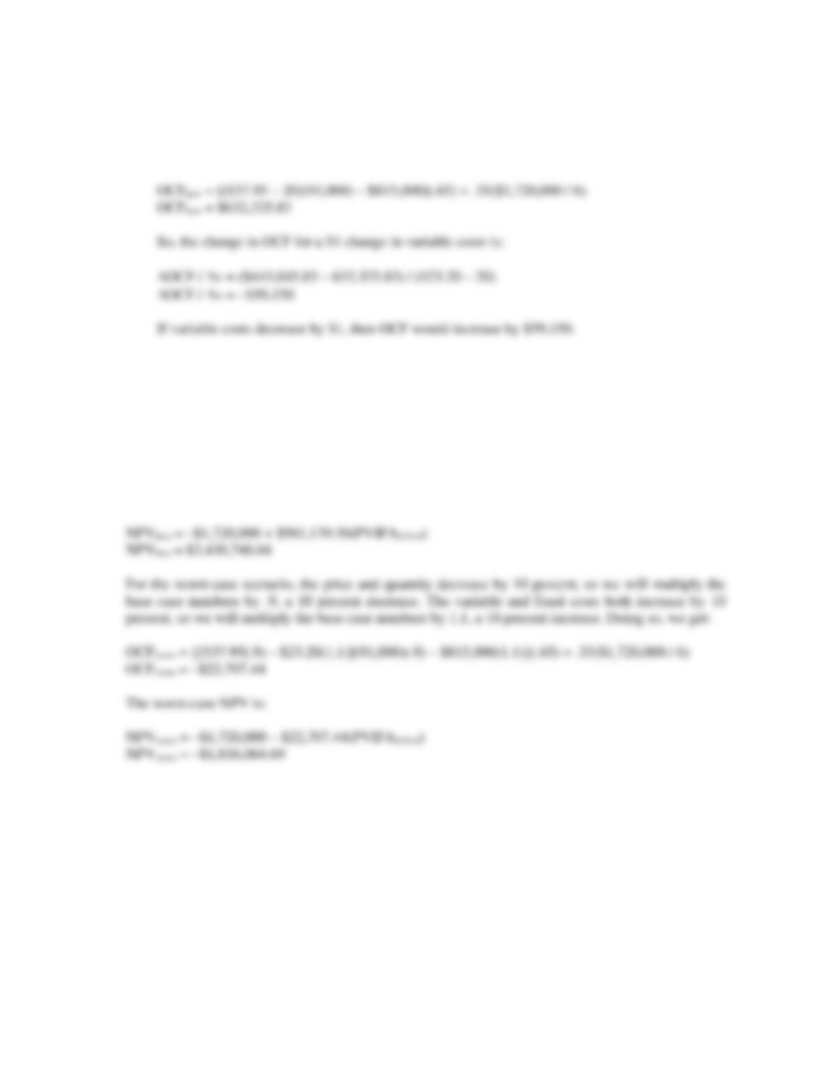
OCFnew = [($37.95 – 23.20)(92,000) – $815,000](.65) + .35($1,720,000 / 6)
OCFnew = $452,633.33
And the NPV is:
NPVnew = –$1,720,000 + $452,633.33(PVIFA11%,6)
NPVnew = $194,882.45
So, the change in NPV for every unit change in sales is:
CHAPTER 8 – 10
b. To find out how sensitive OCF is to a change in variable costs, we will compute the OCF at a
variable cost of $20. Again, the number we choose to use here is irrelevant: We will get the same
ratio of OCF to a one dollar change in variable cost no matter what variable cost we use. So,
using the tax shield approach, the OCF at a variable cost of $20 is:
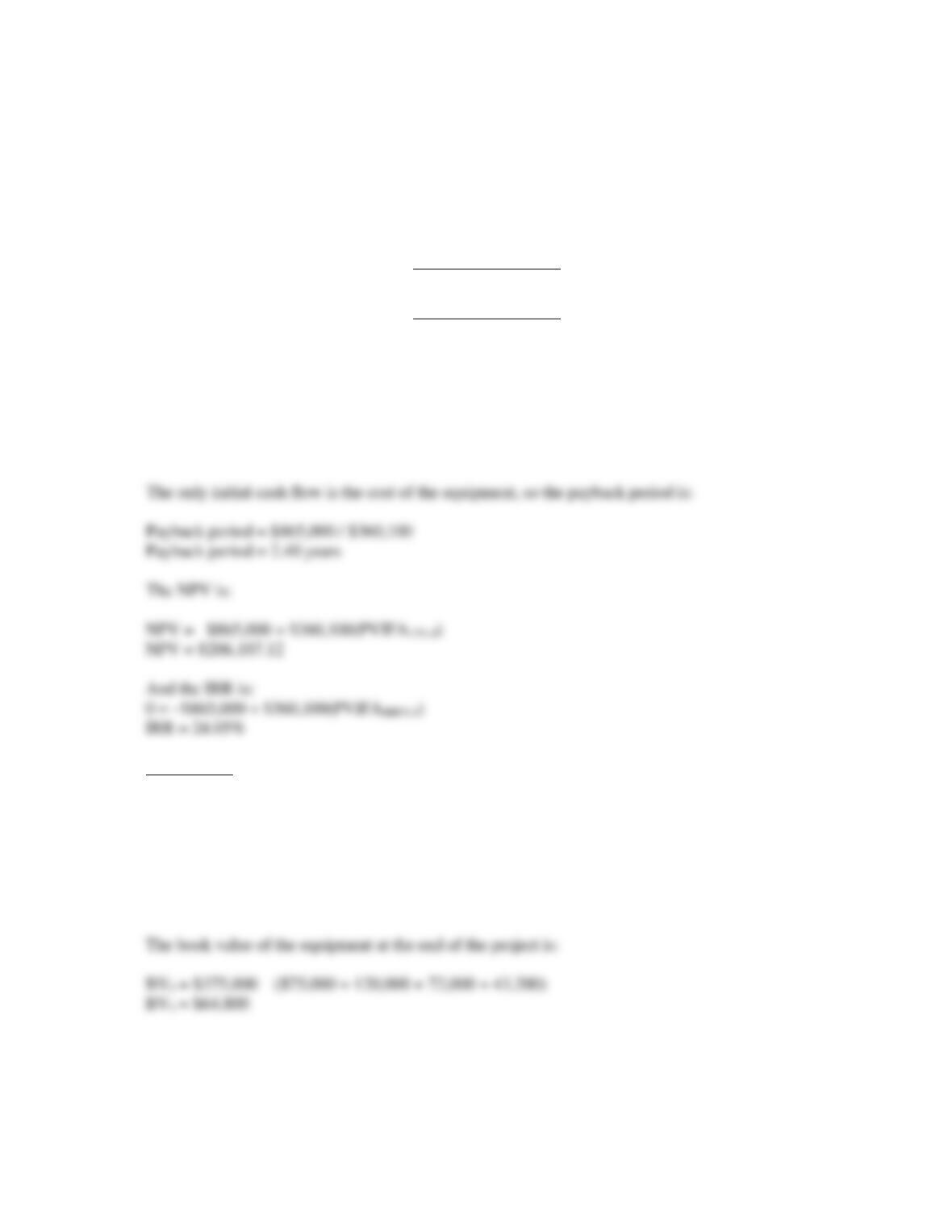
19. We will use the tax shield approach to calculate the OCF for the best– and worst-case scenarios. For
the best-case scenario, the price and quantity increase by 10 percent, so we will multiply the base case
numbers by 1.1, a 10 percent increase. The variable and fixed costs both decrease by 10 percent, so
we will multiply the base case numbers by .9, a 10 percent decrease. Doing so, we get:
OCFbest = {[$37.95(1.1) – $23.20(.9)](91,000)(1.1) – $815,000(.9)}(.65) + .35($1,720,000 / 6)
OCFbest = $981,139.56
The best-case NPV is:
CHAPTER 8 – 11
20. First, we need to calculate the cash flows. The marketing study is a sunk cost and should be ignored.
The net income each year will be:
Sales of new product
$815,000
Variable costs
163,000
Fixed costs
196,000
Depreciation
216,250
EBT
$239,750
Tax
95,900
Net income
$143,850
So, the OCF is:
OCF = EBIT + Depreciation – Taxes
OCF = $239,750 + 216,250 – 95,900
OCF = $360,100
Intermediate
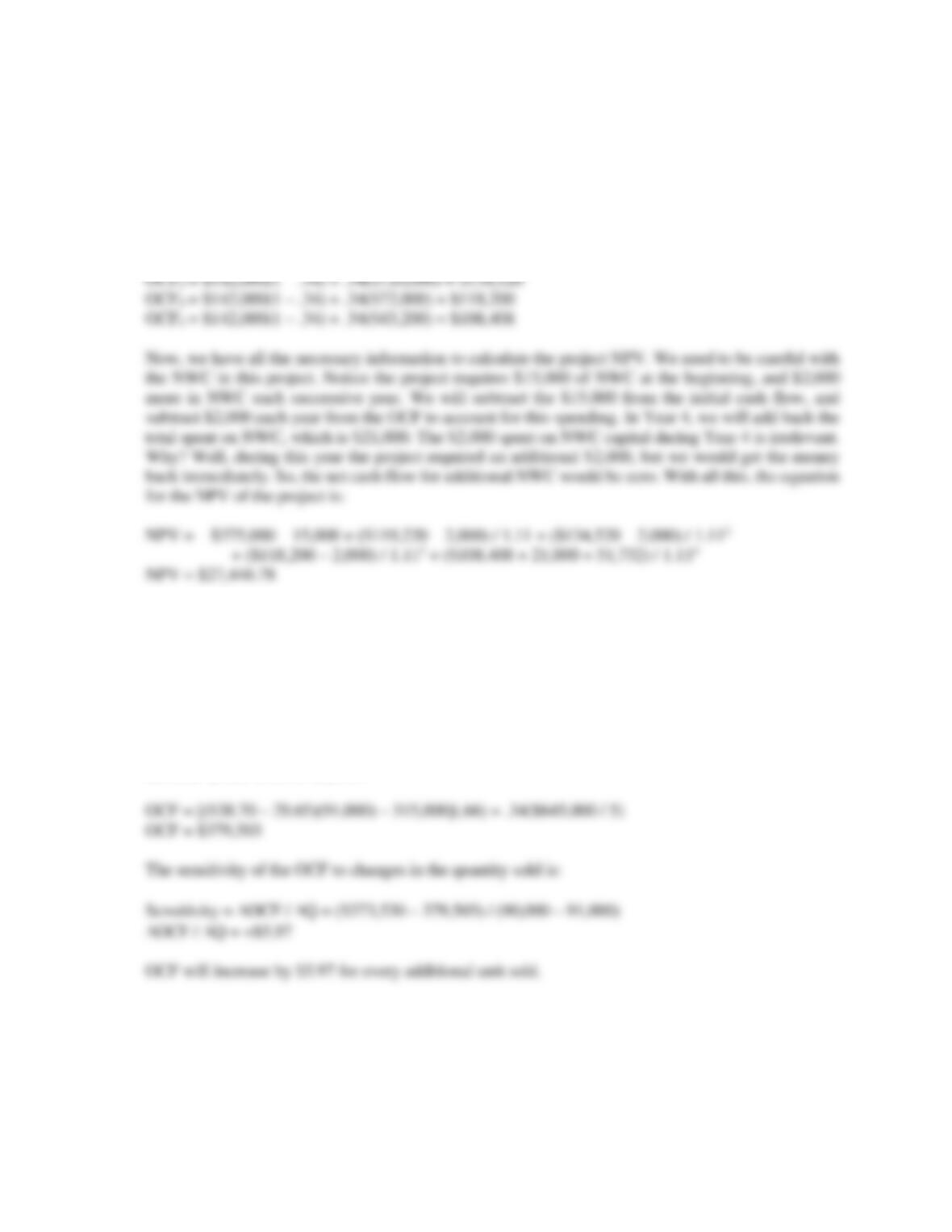
21. First, we will calculate the depreciation each year, which will be:
D1 = $375,000(.2000) = $75,000
D2 = $375,000(.3200) = $120,000
D3 = $375,000(.1920) = $72,000
D4 = $375,000(.1152) = $43,200
CHAPTER 8 – 12
The asset is sold at a loss to book value, so this creates a tax refund.
Aftertax salvage value = $45,000 + ($64,800 – 45,000)(.34)
Aftertax salvage value = $51,732
Using the depreciation tax shield approach, the OCF for each year will be:
OCF1 = $142,000(1 – .34) + .34($75,000) = $119,220
22. Using the tax shield approach, the OCF at 90,000 units will be:
OCF = [(P – v)Q – FC](1 – TC) + Depreciation(TC)
OCF = [($38.70 – 29.65)(90,000) – 315,000](.66) + .34($645,000 / 5)
OCF = $373,530
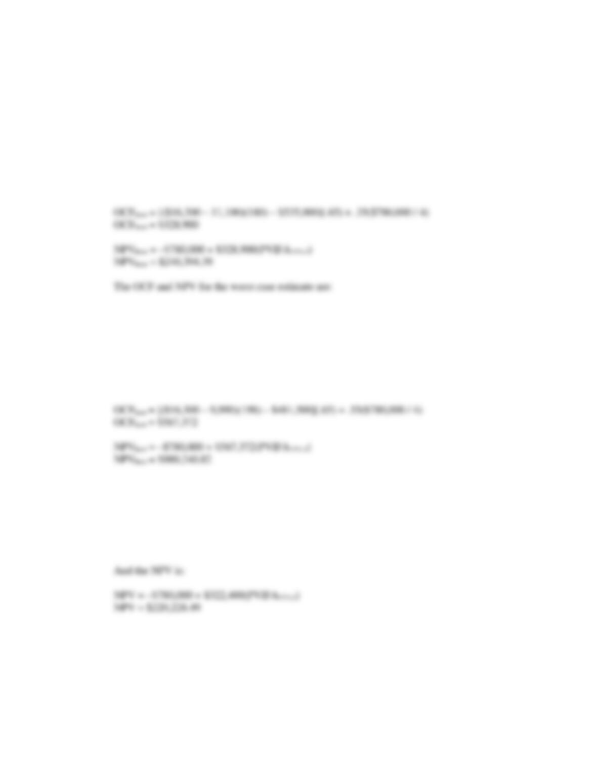
We will calculate the OCF at 91,000 units. The choice of the second level of quantity sold is arbitrary
and irrelevant. No matter what level of units sold we choose, we will still get the same sensitivity. So,
the OCF at this level of sales is:
CHAPTER 8 – 13
23. a. The base-case, best-case, and worst-case values are shown below. Remember that in the best–
case, unit sales increase, while fixed and variable costs decrease. In the worst case, unit sales
decrease, while fixed and variable costs increase.
Scenario Unit sales Variable cost Fixed costs
Base 180 $11,100 $535,000
Best 198 $9,990 $481,500
Worst 162 $12,120 $588,500
Using the tax shield approach, the OCF and NPV for the base case estimate is:
OCFworst = [($16,300 – 12,210)(162) – $588,500](.65) + .35($780,000 / 4)
OCFworst = $116,402
NPVworst = –$780,000 + $116,402(PVIFA11%,4)
NPVworst = –$418,869.12
And the OCF and NPV for the best case estimate are:
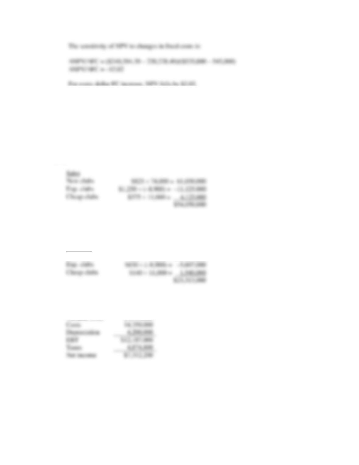
b. To calculate the sensitivity of the NPV to changes in fixed costs, we choose another level of fixed
costs. We will use fixed costs of $545,000. The OCF using this level of fixed costs and the other
base-case values with the tax shield approach, we get:
OCF = [($16,300 – 11,100)(180) – $545,000](.65) + .35($780,000 / 4)
OCF = $322,400
Sales
New clubs
Cheap clubs
CHAPTER 8 – 14
For every dollar FC increase, NPV falls by $2.02.
24. The marketing study and the research and development are both sunk costs and should be ignored.
The initial cost is the equipment plus the net working capital, so:
Initial cost = $29,400,000 + 3,500,000
Initial cost = $32,900,000
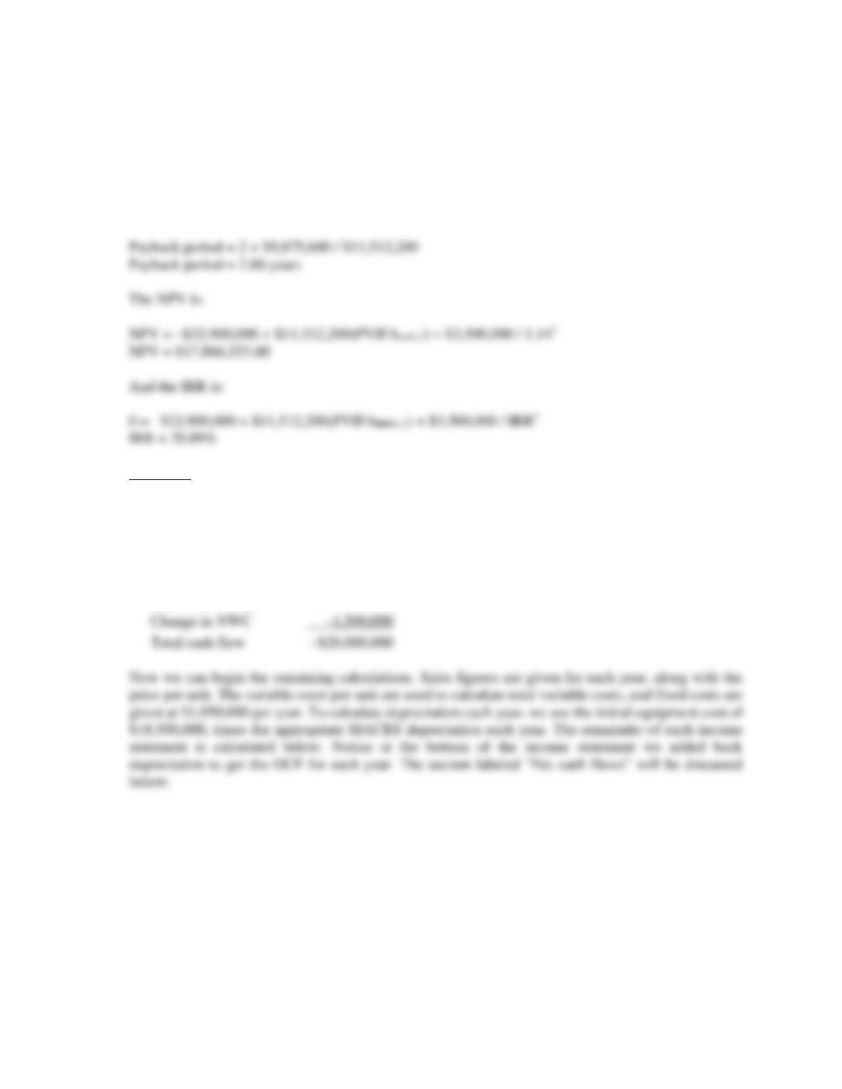
Next, we will calculate the sales and variable costs. Since we will lose sales of the expensive clubs
and gain sales of the cheap clubs, these must be accounted for as erosion. The total sales for the new
project will be:
For the variable costs, we must include the units gained or lost from the existing clubs. Note that the
variable costs of the expensive clubs are an inflow. If we are not producing the sets anymore, we will
save these variable costs, which is an inflow. So:
Var. costs
New clubs
$370 74,000 = $27,380,000
Exp. clubs
The pro forma income statement will be:
Sales
$54,050,000
Variable costs
23,313,000
Costs
Depreciation
EBT
$12,187,000
Taxes
Net income
CHAPTER 8 – 15
Using the bottom up OCF calculation, we get:
OCF = NI + Depreciation
OCF = $7,312,200 + 4,200,000
OCF = $11,512,200
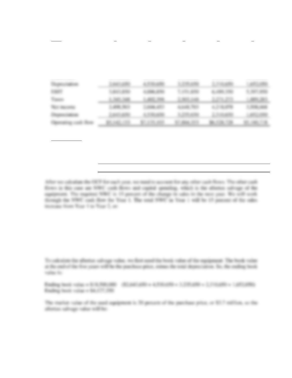
So, the payback period is:
Challenge
25. This is an in-depth capital budgeting problem. We will use the bottom up approach, so we will need
to construct an income statement for each year. Beginning with the initial cash flow at Time 0, the
project will require an investment in equipment. The project will also require an initial investment in
NWC of $1,500,000. So, the cash flow required for the project today will be:
Capital spending
–$18,500,000
CHAPTER 8 – 16
Year
1
2
3
4
5
Ending book value
$15,856,350
$11,325,700
$8,090,050
$5,779,400
$4,127,350
Sales
$23,962,500
$29,784,500
$35,038,500
$30,530,000
$25,560,000
Variable costs
15,525,000
19,297,000
22,701,000
19,780,000
16,560,000
Fixed costs
1,950,000
1,950,000
1,950,000
1,950,000
1,950,000
Net cash flows
Operating cash flow
$5,142,153
$7,135,103
$7,884,353
$6,528,728
$5,160,718
Change in NWC
–873,300
–788,100
676,275
745,500
1,739,625
Capital spending
3,849,573
Total cash flow
$4,268,853
$6,347,003
$8,560,628
$7,274,228
$10,749,915
Change in NWC for Year 1 = .15($23,962,500 – 29,784,500)
Change in NWC for Year 1 = –$873,300
Notice that the NWC cash flow is negative. Since the sales are increasing, we will have to spend more
money to increase NWC. In Year 3, the NWC cash flow is positive since sales are declining. And, in
Year 5, the NWC cash flow is the recovery of all NWC the company still has in the project.
Depreciation
2,643,650
4,530,650
3,235,650
2,310,650
1,652,050
EBIT
3,843,850
4,006,850
7,151,850
6,489,350
5,397,950
Taxes
1,345,348
1,402,398
2,503,148
2,271,273
1,889,283
Net income
2,498,503
2,604,453
4,648,703
4,218,078
3,508,668
Depreciation
2,643,650
4,530,650
3,235,650
2,310,650
1,652,050
Operating cash flow
$5,142,153
$7,135,103
$7,884,353
$6,528,728
$5,160,718
CHAPTER 8 – 17
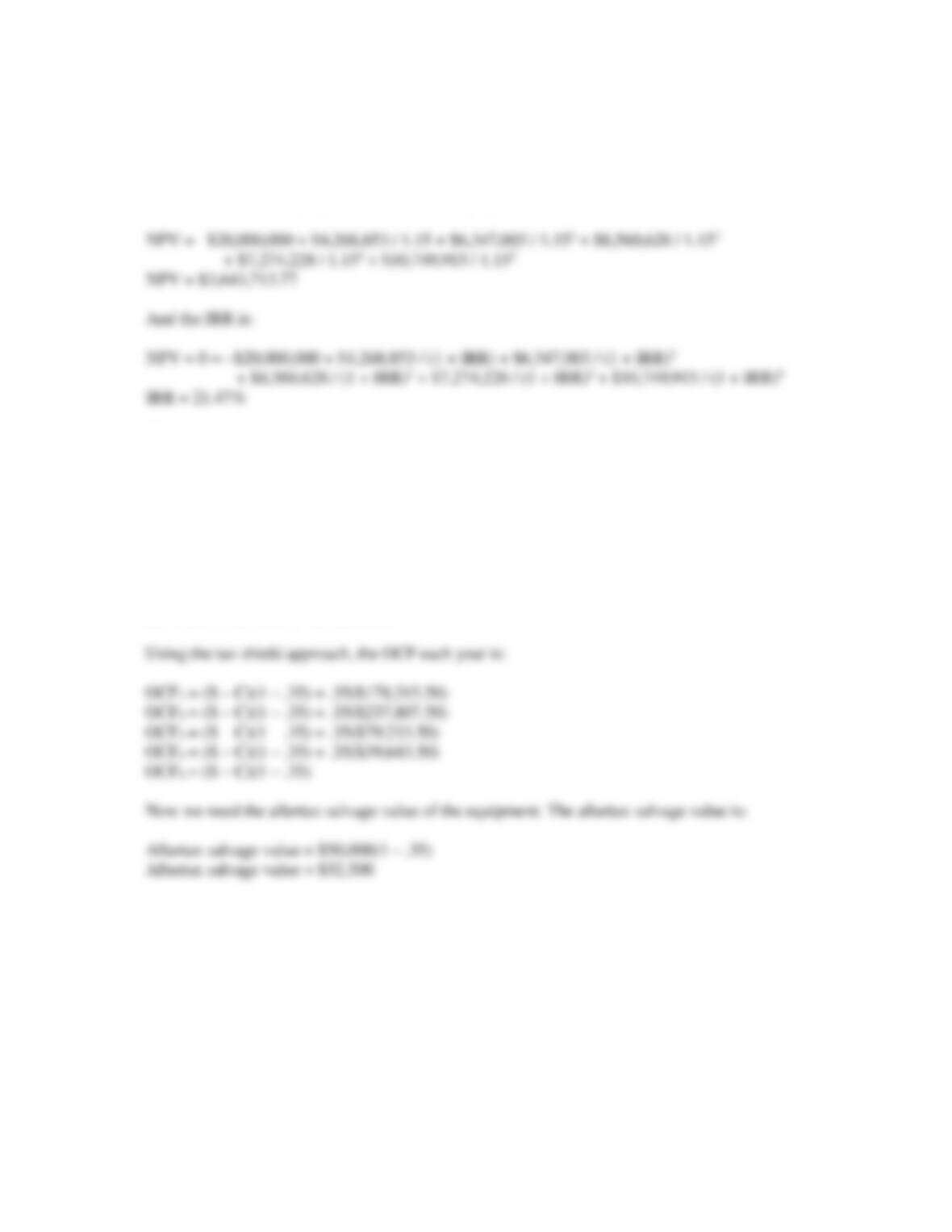
Aftertax salvage value = $3,700,000 + ($4,127,350 – 3,700,000)(.35)
Aftertax salvage value = $3,849,573
The aftertax salvage value is included in the total cash flows as capital spending. Now we have all of
the cash flows for the project. The NPV of the project is:
The company should accept the project.
26. To find the initial pretax cost savings necessary to buy the new machine, we should use the tax shield
approach to find the OCF. We begin by calculating the depreciation each year using the MACRS
depreciation schedule. The depreciation each year is:
D1 = $535,000(.3333) = $178,315.50
D2 = $535,000(.4445) = $237,807.50
D3 = $535,000(.1481) = $79,233.50
D4 = $535,000(.0741) = $39,643.50
CHAPTER 8 – 18
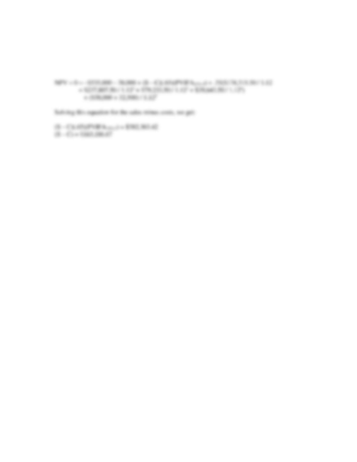
To find the necessary cost reduction, we must realize that we can split the cash flows each year. The
OCF in any given year is the cost reduction (S – C) times one minus the tax rate, which is an annuity
for the project life, and the depreciation tax shield. To calculate the necessary cost reduction, we would
require a zero NPV. The equation for the NPV of the project is: