PROBLEM 8.12 (Cont.)
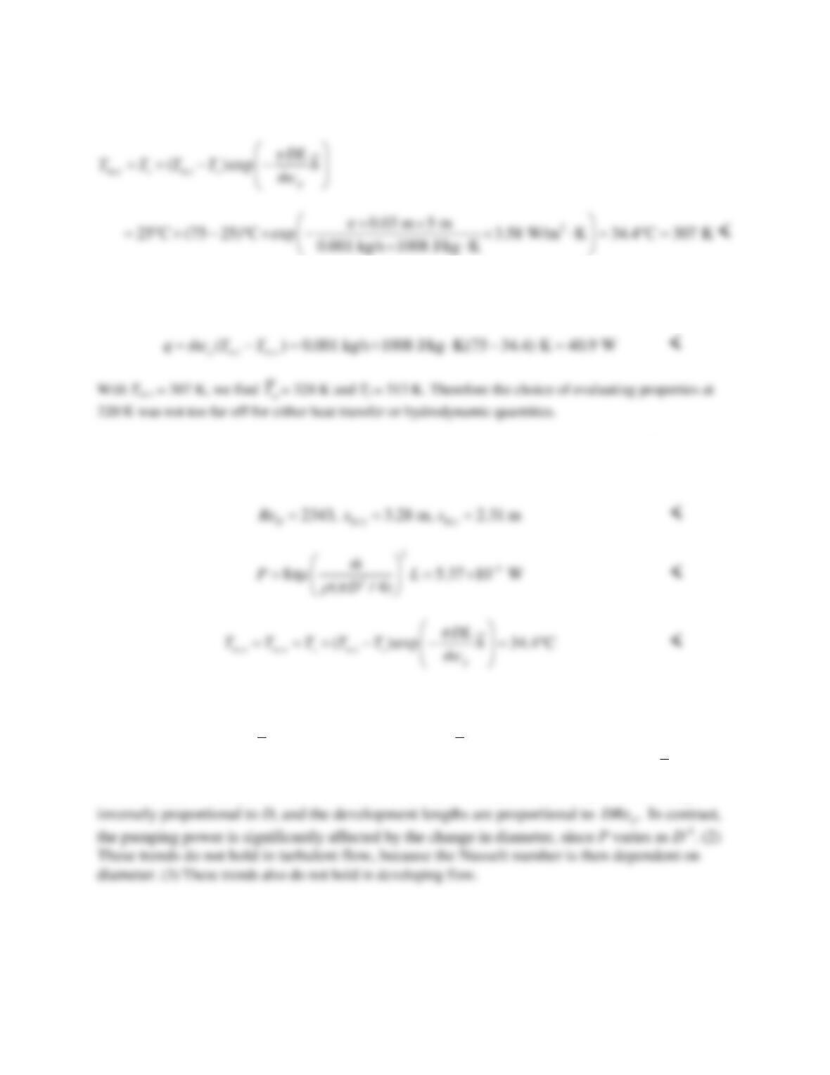
The mean outlet temperature can be found from Equation 8.41b:
The heat transfer rate can be calculated from Equation 8.34 (with a change in sign to calculate heat
transfer from the air to the tube wall):
(b) When the diameter is reduced to 28 mm, the heat transfer coefficient is 3.58 W/m2⋅K(30
mm/28 mm) = 3.84 W/m2⋅K. The calculations can be repeated to find:
and
40.9 Wq=
<
COMMENTS: (1) Since
h
is inversely proportional to D,
hD
is constant. This is typically true for fully
developed laminar flow because the Nusselt number is constant under those conditions. With
hD
constant, Tm,o is unchanged, as is q. Similarly, the development lengths are unchanged because D
Re
is
PROBLEM 8.13
KNOWN: Internal flow with prescribed wall heat flux as a function of distance.
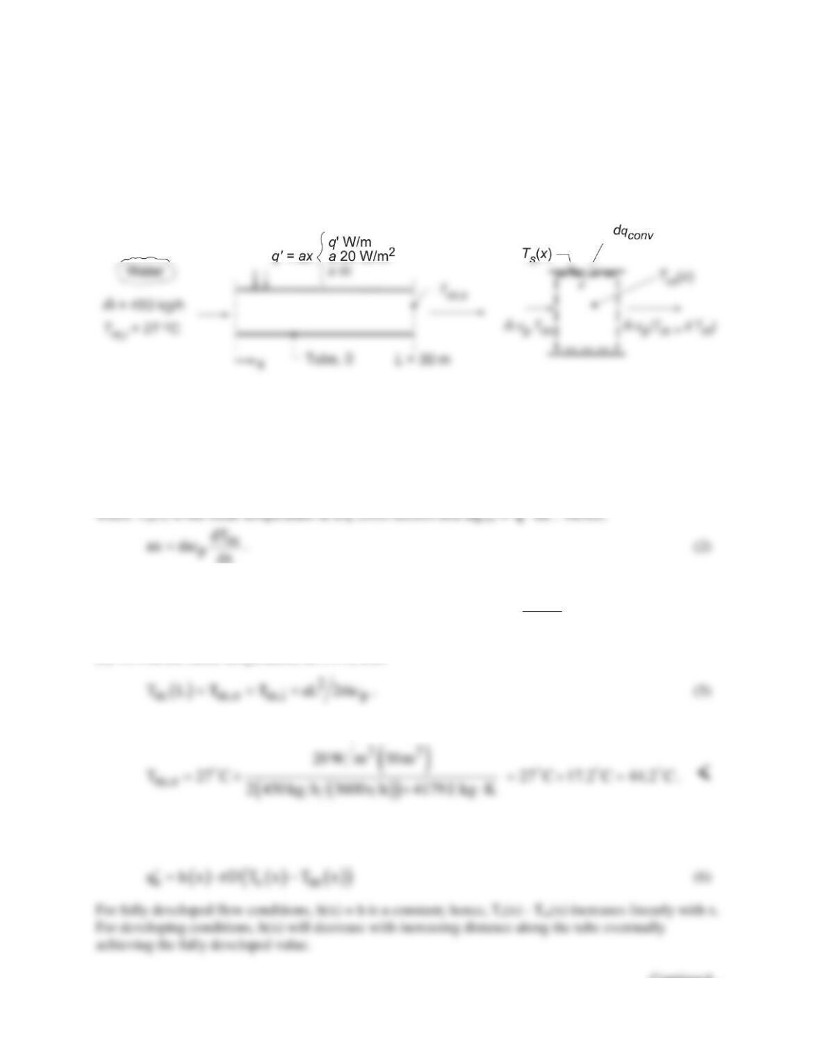
FIND: (a) Beginning with a properly defined differential control volume, the temperature distribution,
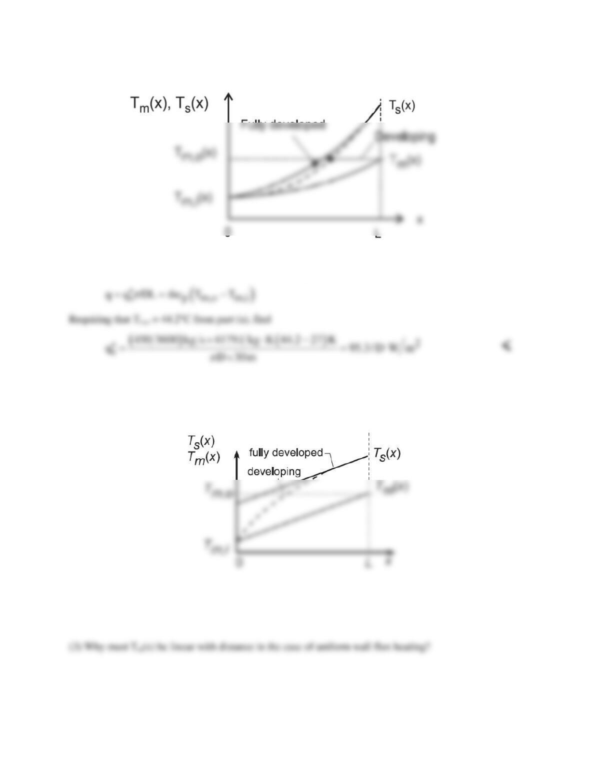
Tm(x), (b) Outlet temperature, Tm,o, (c) Sketch Tm(x), and Ts(x) for fully developed and developing flow
conditions, and (d) Value of uniform wall flux
s
q′′
(instead of
s
q′
= ax) providing same outlet
temperature as found in part (a); sketch Tm(x) and Ts(x) for this heating condition.
SCHEMATIC:
ASSUMPTIONS: (1) Steady-state conditions, (2) Constant properties, (3) Incompressible liquid with
negligible viscous dissipation.
PROPERTIES: Table A.6, Water (300 K): cp = 4.179 kJ/kg⋅K.
ANALYSIS: (a) Applying energy conservation to the control volume above,
conv p m
dq mc dT=
(1)
′⋅
Separating and integrating with proper limits gives
( )
m
m,i
x Tx
pm
x0 T
a xdx mc dT
==
∫∫
( )
2
m m,i p
ax
Tx T 2mc
= +
(3,4)<
(b) To find the outlet temperature, let x = L, then
Solving for Tm,o , we find
(c) For linear wall heating,
s
q =ax
′
, the fluid temperature distribution along the length of the tube is
quadratic as prescribed by Eq. (4). From the convection rate equation,
Continued…
PROBLEM 8.13 (Cont.)
(d) For uniform wall heat flux heating, the overall energy balance on the tube yields
where D is the diameter (m) of the tube which, when specified, would permit determining the required
heat flux,
s
q′′
. For uniform heating, Section 8.3.2, we know that Tm(x) will be linear with distance. Ts(x)
will also be linear for fully developed conditions and appear as shown below when the flow is
developing.
COMMENTS: (1) Note that cp should be evaluated at Tm = (27 + 44)°C/2 = 309 K.
(2) Why did we show Ts(0) = Tm(0) for both types of history when the flow was developing?
PROBLEM 8.14
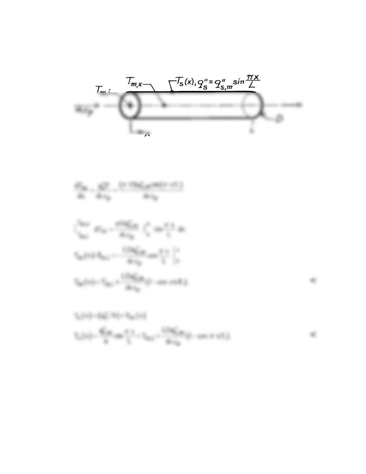
KNOWN: Geometry and coolant flow conditions associated with a nuclear fuel rod. Axial
variation of heat generation within the rod.
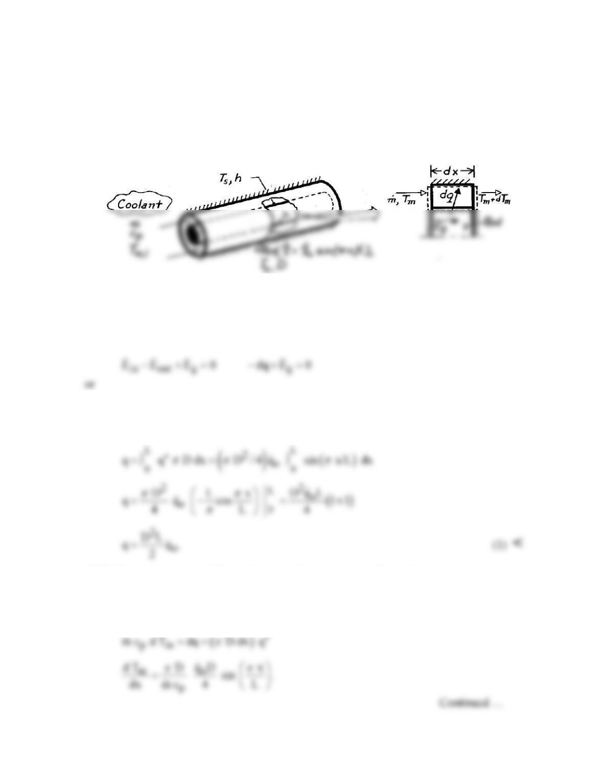
FIND: (a) Axial variation of local heat flux and total heat transfer rate, (b) Axial variation of
mean coolant temperature, (c) Axial variation of rod surface temperature and location of
maximum temperature.
SCHEMATIC:
ASSUMPTIONS: (1) Steady-state conditions, (2) Constant fluid properties, (3) Uniform
surface convection coefficient, (4) Negligible axial conduction in rod and fluid, (5)
Incompressible liquid with negligible viscous dissipation, (6) Outer surface is adiabatic.
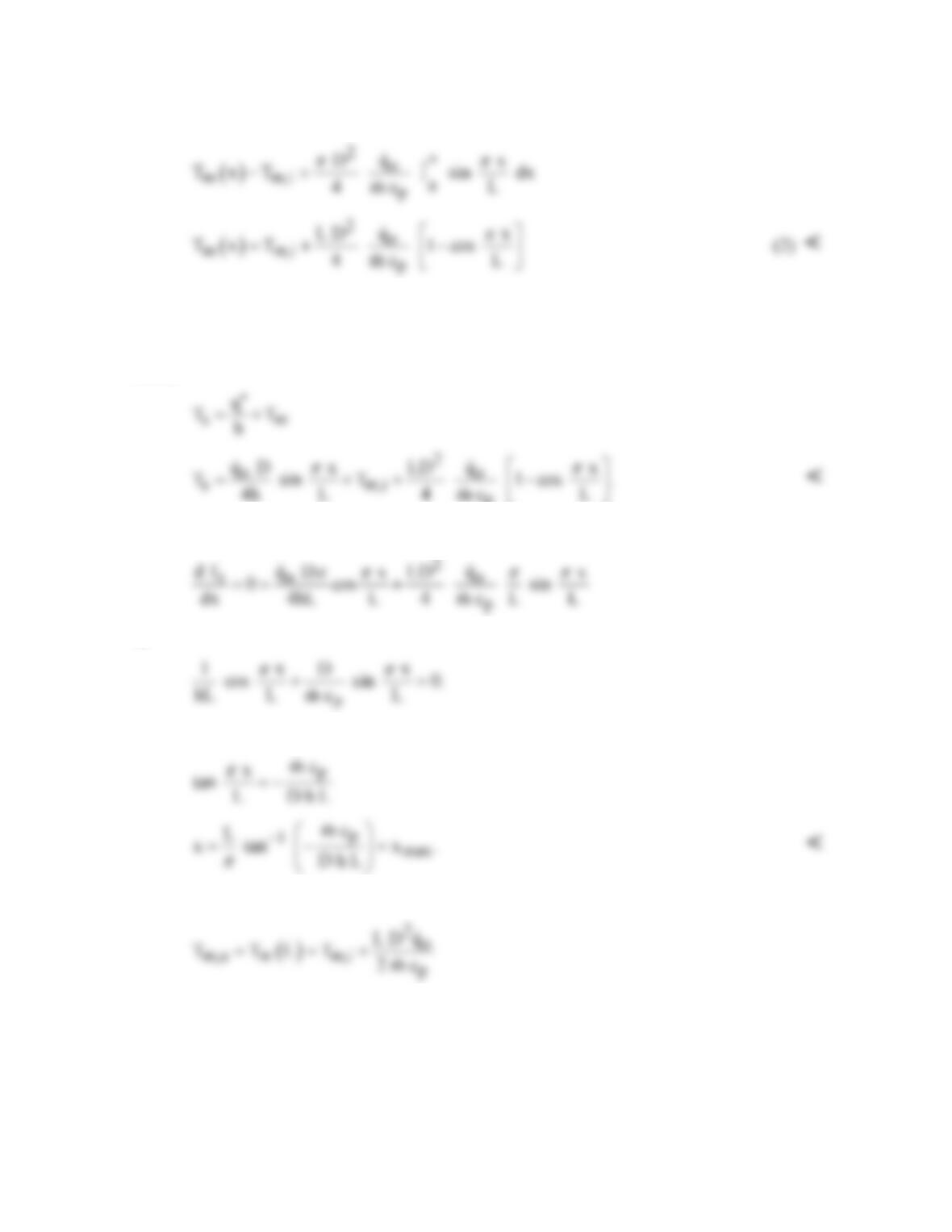
ANALYSIS: (a) Performing an energy balance for a control volume about the rod,
( ) ( )
()
( ) ( )
2
oo
q D dx q sin x/L D / 4 dx=0 q q D/4 sin x/L .
π ππ π
′′ ′′
−+ =
<
The total heat transfer rate is then
(b) Performing an energy balance for a control volume about the coolant,
( )
pm p m m
m c T dq m c T dT 0.+= + =
Hence
PROBLEM 8.14 (Cont.)
Integrating,
(c) From Newton’s law of cooling,
( )
sm
q hT T .
′′ = −
Hence
To determine the location of the maximum surface temperature, evaluate
or
Hence
COMMENTS: Note from Eq. (2) that
which is equivalent to the result obtained by combining Eq. (1) and Eq. 8.34.
PROBLEM 8.15
KNOWN: Axial variation of surface heat flux for flow through a tube.
FIND: Axial variation of fluid and surface temperatures.
SCHEMATIC:
ASSUMPTIONS: (1) Convection coefficient is independent of x, (2) Applicability of Eq.
8.34.
ANALYSIS: Since Equation 8.37 is applicable,
Separating variables and integrating from x = 0
From Newton’s law of cooling, Eq. 8.27,
COMMENTS: For the prescribed surface condition, the flow is not fully developed. Hence,
the assumption of constant h should be viewed as a first approximation.
PROBLEM 8.16
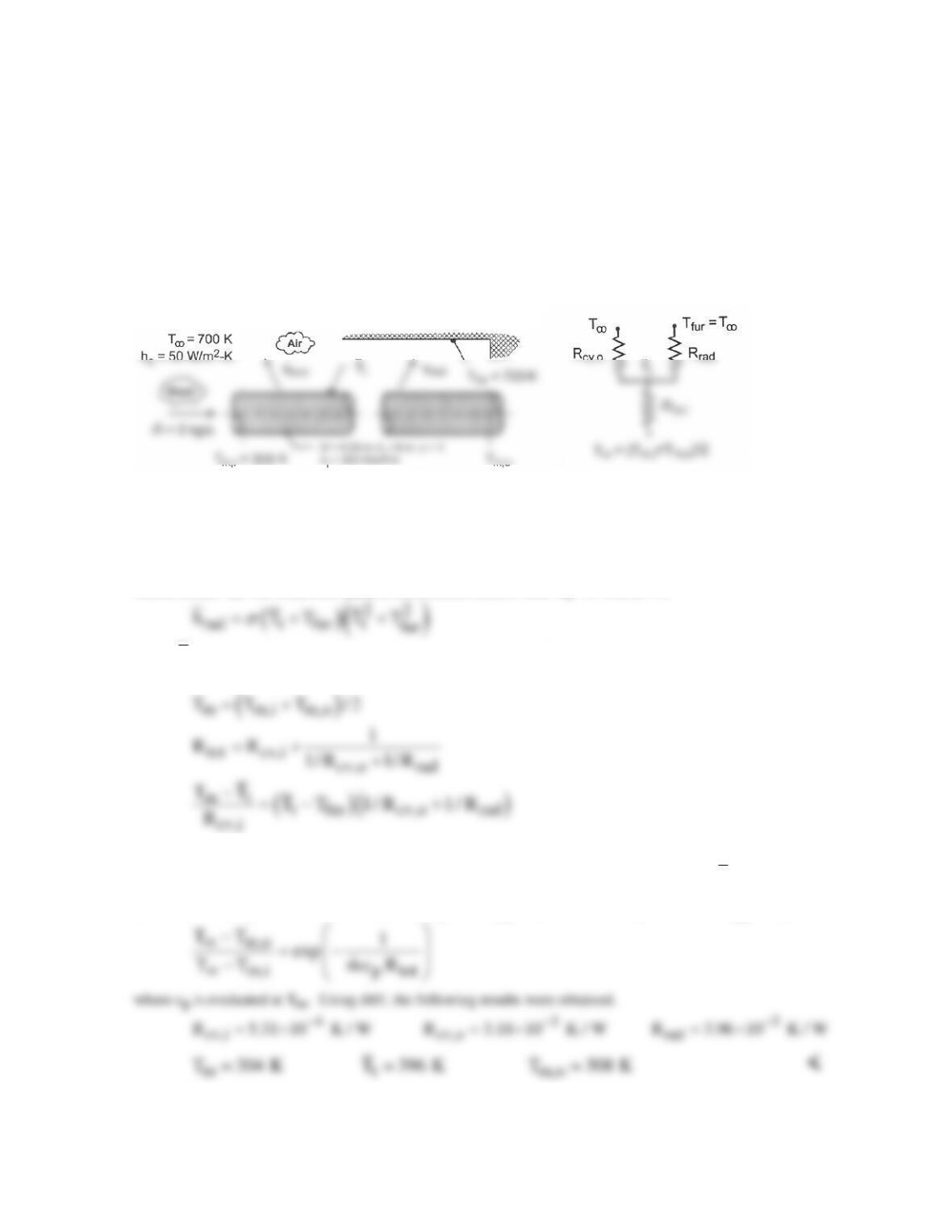
KNOWN: Water at prescribed temperature and flow rate enters a 0.25 m diameter, black thin-walled tube of 8-
m length, which passes through a large furnace whose walls and air are at a temperature of Tfur = T∞ = 700 K.
The convection coefficients for the internal water flow and external furnace air are 300 W/m2⋅K and 50 W/m2⋅K,
respectively.
FIND: (a) An expression for the linearized radiation coefficient for the radiation exchange process between the
outer surface of the pipe and the furnace walls; represent the tube by an average temperature and explain how to
calculate this value, and (b) determine the outlet temperature of the water, To.
SCHEMATIC:
ASSUMPTIONS: (1) Steady-state conditions; (2) Tube is small object with large, isothermal surroundings; (3)
Furnace air and walls are at the same temperature; (4) Tube is thin-walled with black surface; and (5)
Incompressible liquid with negligible viscous dissipation.
PROPERTIES: Table A-6, Water (Tm = (Tm,i + Tm,o)/2 = 304 K): cp = 4178 J/kg⋅K.
ANALYSIS: (a) The linearized radiation coefficient follows from Eq. 1.9 with ε = 1,
where t
T represents the average tube wall surface temperature, which can be evaluated from an energy balance
on the tube as represented by the thermal circuit above.
The thermal resistances, with As = PL = πDL, are
cv,i i s cv,o o s rad rad s
R1/hA R 1/hA R1/hA===
(b) The outlet temperature can be calculated using the energy balance relation, Eq. 8.45b, with Tfur = T∞,
COMMENTS: Since T∞ = Tfur, it was possible to use Eq. 8.45b with Rtot. How would you write the energy
balance relation if T∞ Tfur?
PROBLEM 8.17
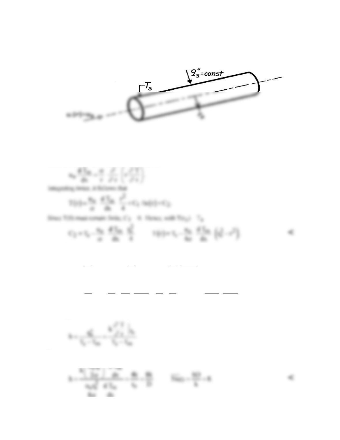
KNOWN: Laminar, slug flow in a circular tube with uniform surface heat flux.
FIND: Temperature distribution and Nusselt number.
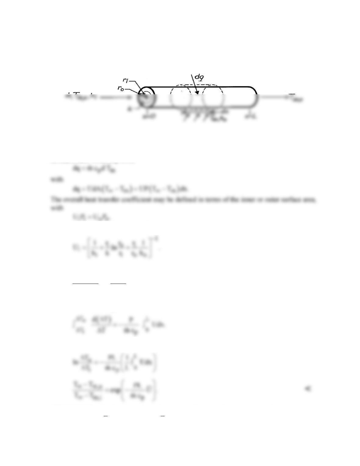
SCHEMATIC:
ASSUMPTIONS: (1) Steady, incompressible flow, with negligible viscous dissipation, (2) Constant
properties, (3) Fully developed, laminar flow, (4) Uniform surface heat flux.
ANALYSIS: With v = 0 for fully developed flow and ∂T/∂x = dTm/dx = const, from Eqs. 8.32 and
8.39, the energy equation, Eq. 8.48, reduces to
From Eq. 8.26, with um = uo,
()
rr
oo
00
23
om
m so
22
oo
u
2 2 d T
T Tr dr T r rr r dr
4 dx
rr
=∫ =∫− −
2 44 2
o o o o oo
mm
ms s
2
o
r u r r ur
2 d T d T
T T T .
2 4 dx 2 4 8 dx
r
= − −=−
From Eq. 8.27 and Fourier’s law,
hence,
PROBLEM 8.18
KNOWN: Heat transfer between fluid flow over a tube and flow through the tube.
FIND: Axial variation of mean temperature for inner flow.
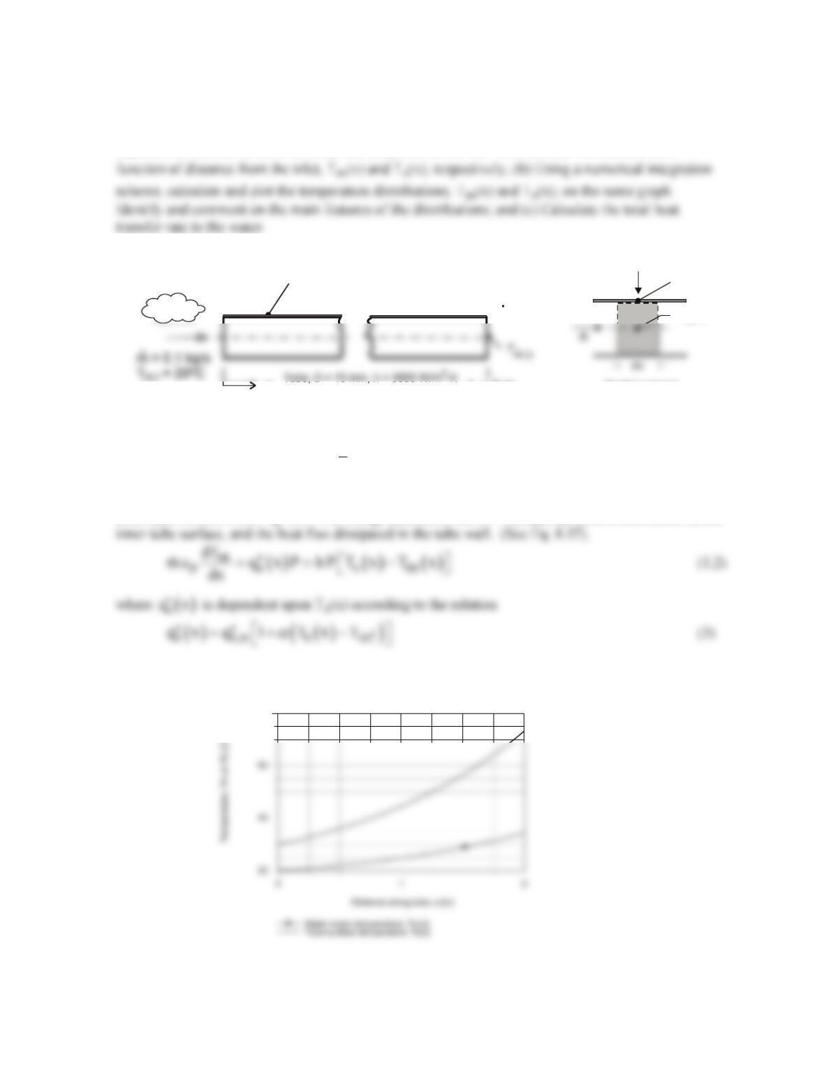
SCHEMATIC:
ASSUMPTIONS: (1) Applicability of Eq. 8.34, (2) Negligible axial conduction, (3)
Constant cp, (4) Uniform T∞.
ANALYSIS: From Eq. 8.36,
For the inner surface, from Eq. 3.36,
Hence,
m
mp
d T UP dx
T T m c
∞
= +
−
or, with ∆T ≡ T∞ – Tm,
Hence,
COMMENTS: The development and results parallel those for a constant surface
temperature, with
s
U and T replacing h and T .
∞
PROBLEM 8.19
KNOWN: Water is heated in a tube having a wall flux that is dependent upon the wall temperature.
FIND: (a) Beginning with a properly defined differential control volume in the tube, derive
expressions that can be used to obtain the temperatures for the water and the wall surface as a
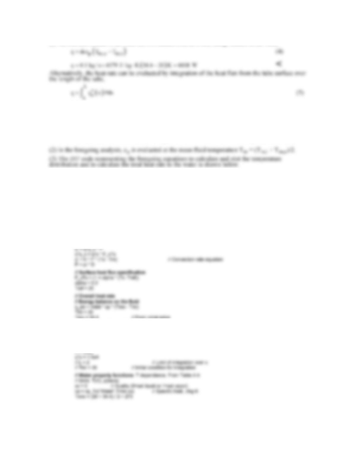
SCHEMATIC:
Water
q” (x) = q” [1+ (T – T )]
s ref
s,o
s
T (x)
m
T (x)
s
dq
cv
= 0.2 K
-1
q” = 1×10 W/m
42
s,o
= T 20 C
ref o
L = 2 m
xControl volume
ASSUMPTIONS: (1) Steady-state conditions, (2) Fully developed flow and thermal conditions, (3)
No losses to the outer surface of the tube, (3) Constant properties, and (4) Incompressible liquid with
negligible viscous dissipation .
PROPERTIES: Table A-6, Water
( )
( )
m m,i m,o
T T T / 2 300 K :=+=
cp = 4179 J/kg⋅K
ANALYSIS: (a) The properly defined control volume of perimeter P = πD shown in the above
schematic follows from Fig. 8.6. The energy balance on the CV includes advection, convection at the
(b) Eqs. (1 and 2) with Eq. (3) can be solved by numerical integration using the Der function in IHT
as shown in Comment 1. The temperature distributions for the water and wall surface are plotted
below.
Continued …
80
PROBLEM 8.19 (Cont.)
(c) The total heat transfer to the water can be evaluated from an overall energy balance on the water,
where
( )
s
qx
′′
is given by Eq. (3), and Ts(x) and Tm(x) are determined from the differential form of
the energy equation, Eqs. (1) and (2). The result as shown in the IHT code below is 6005 W.
COMMENTS: (1) Note that Tm(x) increases with distance greater than linearly, as expected since
s
q (x)
′′
does. Also as expected, the difference, Ts(x) – Tm(x), likewise increases with distance greater than linearly.
/* Results: integration for distributions; conditions at x = 2 m
F_xTs Ts q’ q”s_x x Tm
11.64 73.18 5483 1.164E5 2 34.39
3 30 1414 3E4 0 20 */
/* Results: heat rate by energy balances on fluid and tube surface
q_eb q_hf
6018 6005 */
/* Results: for evaluating cp at Tm
Ts cp q”s_x x Tm
73.31 4179 1.166E5 2 34.44
30 4179 3E4 0 20 */
// Energy balances
mdot * cp * der(Tm,x) = q’ // Energy balance, Eq. 8.37
Tmo = 34.4 // From initial solve
// Integration of the surface heat flux
q_hf = q”o * P * INTEGRAL(F_xTs, x)
// Input variables
mdot = 0.1
D = 0.015
PROBLEM 8.20
KNOWN: Inlet temperature and flowrate of oil moving through a tube of prescribed diameter and
surface temperature.
FIND: (a) Oil outlet temperature Tm,o for two tube lengths, 5 m and 100 m, and log mean and arithmetic
mean temperature differences, (b) Effect of L on Tm,o and
D
Nu
.
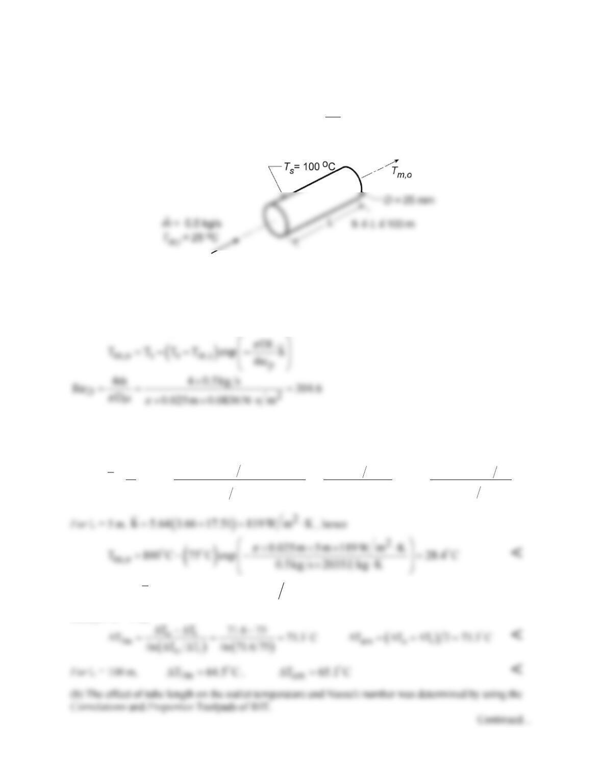
SCHEMATIC:
ASSUMPTIONS: (1) Steady-state conditions, (2) Incompressible liquid with negligible viscous
dissipation, (3) Constant properties.
PROPERTIES: Table A.4, Oil (330 K): cp = 2035 J/kg⋅K, m = 0.0836 N⋅s/m2, k = 0.141 W/m⋅K, Pr =
1205.
ANALYSIS: (a) Using Eqs. 8.41b and 8.6
With xfd,h = 0.05DReD = 0.4 m, it is reasonable to assume the flow is hydrodynamically fully developed.
However, with xfd,t = xfd,h Pr = 495 m, the flow is thermally developing. Since thermal entry length effects
will be significant and Pr > 5, use Eq. 8.57 with Eq. 8.56 for the Graetz number:
( )
( ) ( )
4
D
2/3 2/3
D
0.0688 D L Re Pr
k 0.141W m K 2.45 10 D L
h 3.66 3.66
D 0.025m 1 205 D L
1 0.04 D L Re Pr
⋅×
=+=+
+
+
For L = 100 m,
( )
2
h 5.64 3.66 3.38 40 W m K= += ⋅
, Tm,o = 44.9°C. <
Also, for L = 5 m,
PROBLEM 8.20 (Cont.)
45
50
20
25
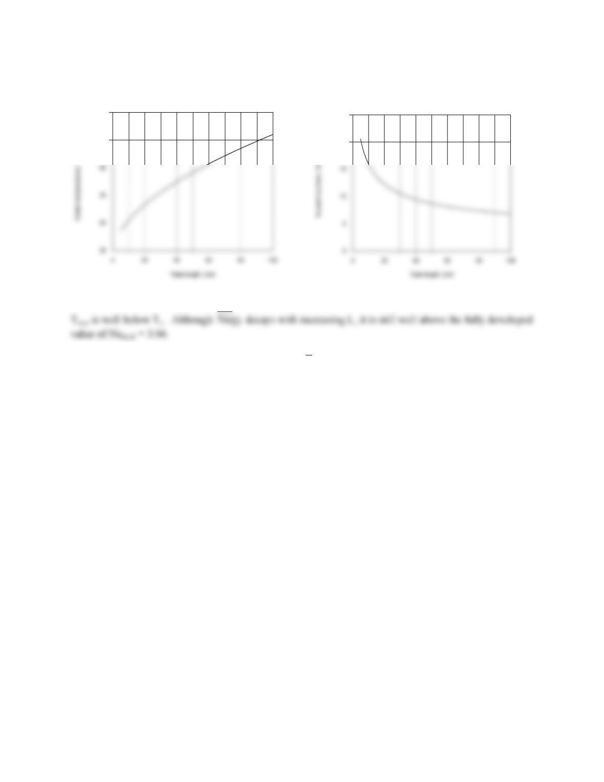
The outlet temperature approaches the surface temperature with increasing L, but even for L = 100 m,
COMMENTS: (1) The average, mean temperature,
m
T
= 330 K, was significantly overestimated in
part (a). The accuracy may be improved by evaluating the properties at a lower temperature. (2) Use of
∆Tam instead of
m
T∆
is reasonable for small to moderate values of (Tm,i – Tm,o ). For large values of
(Tm,i – Tm,o ),
m
T∆
should be used.
PROBLEM 8.21
KNOWN: Inlet and outlet temperatures and velocity of fluid flow in tube. Tube diameter and length.
FIND: Surface heat flux and temperatures at x = 0.5 and 10 m.
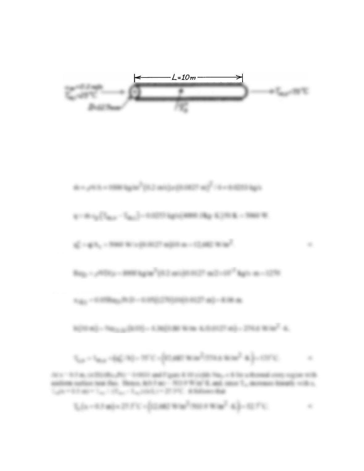
SCHEMATIC:
ASSUMPTIONS: (1) Steady-state conditions, (2) Constant properties, (3) Negligible heat loss to
surroundings, (4) Incompressible liquid with negligible viscous dissipation, (5) Negligible axial
conduction.
PROPERTIES: Pharmaceutical (given): ρ = 1000 kg/m3, cp = 4000 J/kg⋅K, m = 2 × 10⁻³ kg/s⋅m, k =
0.80 W/m⋅K, Pr = 10.
ANALYSIS: With
Eq. 8.34 yields
The required heat flux is then
With
the flow is laminar and Eq. 8.23 yields
Hence, with fully developed hydrodynamic and thermal conditions at x = 10 m, Eq. 8.53 yields
Hence, from Newton’s law of cooling,
PROBLEM 8.22
KNOWN: Laminar boundary layer development in a tube entrance.
FIND: (a) Expression for NuD in terms of
1
D
Gz
−
and Pr. Plot of NuD versus
1
D
Gz
−
for Pr = 0.7. (b)
Expression for
D
Nu
in terms of
1
D
Gz−
and Pr. Comparison to combined entrance length correlation in
the limit of small x.
SCHEMATIC:
ASSUMPTIONS: (1) Constant properties. (2) Laminar conditions.
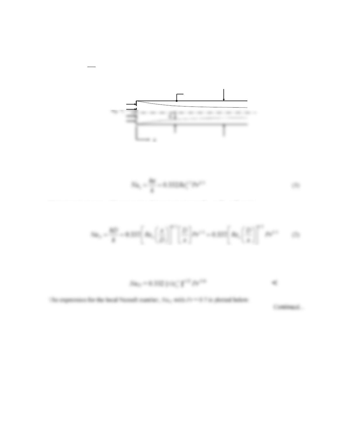
ANALYSIS: (a) From Equation 7.23, the Nusselt number based upon the streamwise coordinate x is
Multiplying both sides of Equation 1 by D/x and substituting Rex = ReDx/D yields
Substituting
1
D
Gz−
= (x/D)/(ReDPr) into Equation 2 and noting that Pr1/3 = Pr1/2⋅Pr–1/6 yields
Ts
D
PROBLEM 8.22 (Cont.)
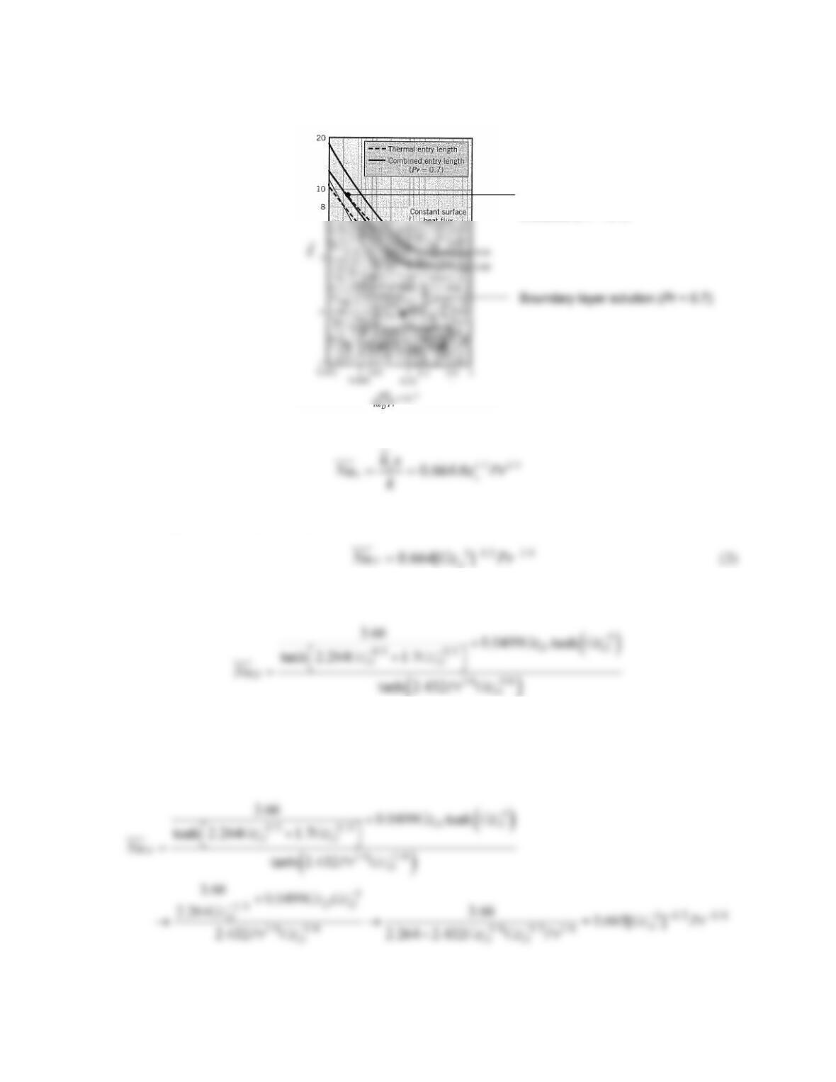
(b) Equation 7.30 gives the following for the average Nusselt number:
Following the same steps as in part (a), this can be rewritten as
The average Nusselt number for the combined entrance length is given as
In the limit of small x,
1
D
Gz
−
is also small. Furthermore,
2/3 1/3
DD
Gz Gz
−−
<<
Noting that tanh(
ε
) →
ε
as
ε
→ 0, we find
This is in excellent agreement with Eq. (3).
Continued…
Combined thermal
entrance (Pr = 0.7)

PROBLEM 8.22 (Cont.)
COMMENT: The combined thermal entrance length solution and the boundary layer solution based
D
PROBLEM 8.23
KNOWN: Tube length, diameter and surface temperature. Mass flow rate and inlet temperature of
fluid.
FIND: (a) Heat transfer rate if the fluid is water. (b) Heat transfer rate for the nanofluid of Example
2.2.
SCHEMATIC:
ASSUMPTIONS: (1) Constant properties, (2) Negligible viscous dissipation.
PROPERTIES: Table A.4, water (300 K):
m
bf = 855 × 10-6 m2/s, kbf = 0.613 W/m⋅K, cp,bf = 4179
ANALYSIS: (a) The Reynolds number is
Therefore the flow is laminar. The hydrodynamic and thermal entry lengths are
Since the tube length is L = 8 m, the temperature is still developing. The hydrodynamic entry length is
less than the tube length, but perhaps not sufficiently shorter to consider the velocity to be fully
developed through the entire tube. With Prbf > 5, the Hausen correlation, Equation 8.57, could be used
as an approximation. However the nanofluid Prandtl number is less than 5. To compare the two fluids
on an equal basis, we will use the combined entry correlation, Equation 8.58, for both. With GzD =
Ts = 30°C
D = 15 mm
D= 20 mm
PROBLEM 8.23 (Cont.)
Therefore the heat transfer rate to the water is
(b) The preceding calculations may be repeated for the nanofluid. The results are:
The combined entry solution is again appropriate. The remaining results are:
COMMENTS: (1) The nanofluid of Example 2.2 is water containing Al2O3 nanoparticles. The
thermal conductivity of the nanofluid is 15% greater than that of the base fluid (water). In addition, the
convection heat transfer coefficient of the nanofluid is 8% greater than that of the water, and the
PROBLEM 8.24
KNOWN: Oil at 70°C enters a single-tube preheater of 10-mm diameter and 5–m length; tube surface
maintained at 180°C by swirling combustion gases.
FIND: Determine the flow rate and heat transfer rate when the outlet temperature is 105°C.
SCHEMATIC:
ASSUMPTIONS: (1) Laminar flow, (2) Tube wall is isothermal, (3) Incompressible liquid with
negligible viscous dissipation, (4) Constant properties.
ANALYSIS: The overall energy balance, Eq. 8.34, and rate equation, Eq. 8.41b, are
( )
p m,o m,i
q mc T T= −
(1)
where all properties are evaluated at Tm = (Tm,i + Tm,o )/2. The Reynolds number follows from Eq.
8.6,
D
Re 4m / D
πm
=
(4)
A tedious trial–and-error solution is avoided by using IHT to solve the system of equations with the
following result:
COMMENT: Use of the Baehr and Stephan correlation for the combined entry problem yields the
identical values. Hence it may also be used.
175
175
Ts= 180°C