Chap. 8 Spread Footings-Geotechnical Serviceability Limit States
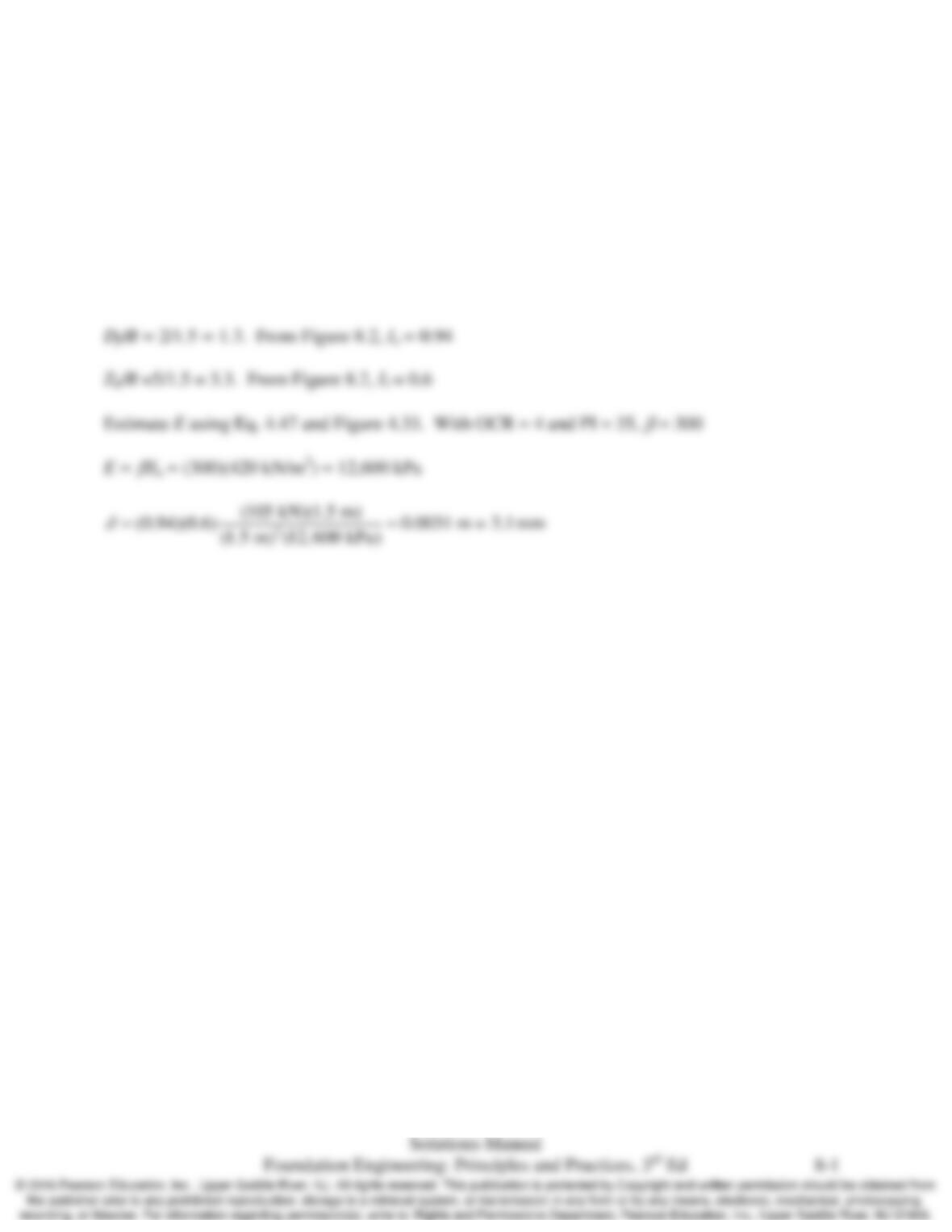
8.1 A 1.5 m square footing and carries a column with a service load of 105 kN. It is founded at a
depth of 2 m on a medium stiff clay with an undrained shear strength of 42 kPa, an
overconsolidation ratio of 4, and a plasticity index of 35. The clay layer is 5 m thick and overlies
a very stiff shale. Estimate the undrained settlement of the footing based using the generalized
elastic method with Christian and Carrier’s (1978) influence factors.
Solution
Determine the influence factors, Io and I1
Chap. 8 Spread Footings-Geotechnical Serviceability Limit States
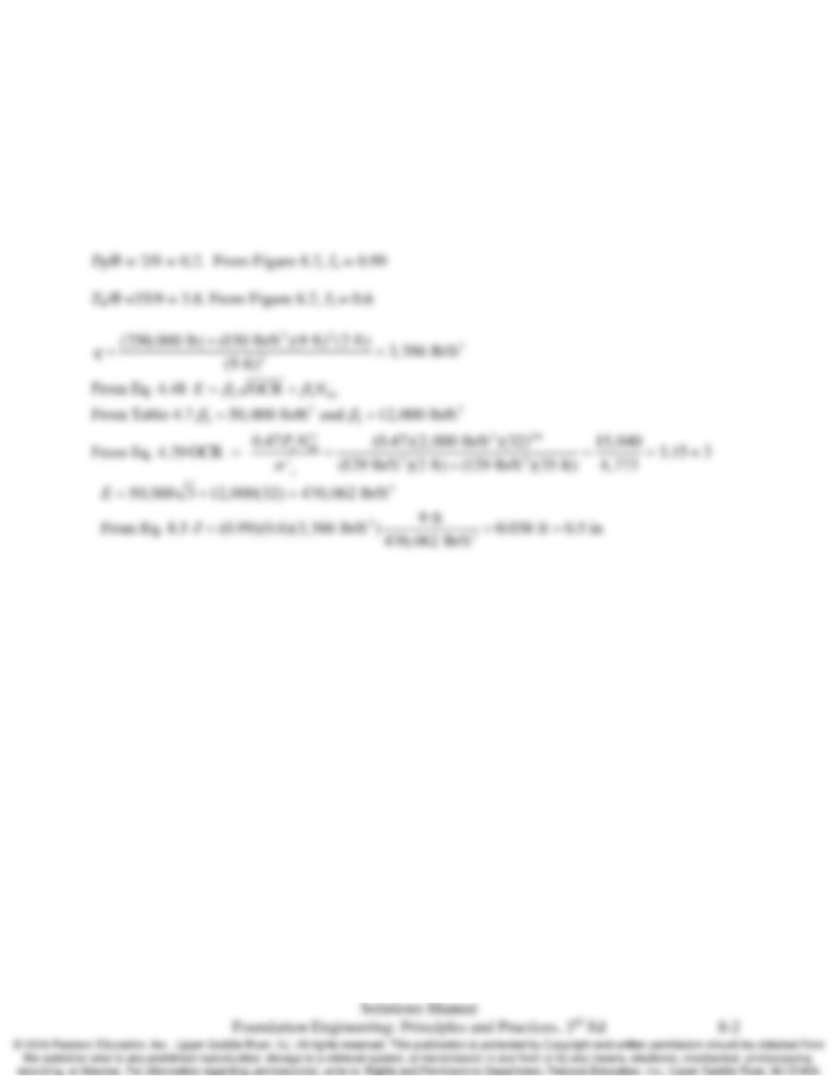
8.2 A 250-k column load is to be supported on a 9 ft square footing embedded 2 ft below the ground
surface. The underlying soil is a silty sand with an average N60 of 32 and a unit weight of
129 lb/ft3. The groundwater table is at a depth of 35 ft. Estimate the undrained settlement of the
footing using the generalized elastic method with Christian and Carrier’s (1978) influence factors.
Solution
Determine the influence factors, Io and I1
Chap. 8 Spread Footings-Geotechnical Serviceability Limit States
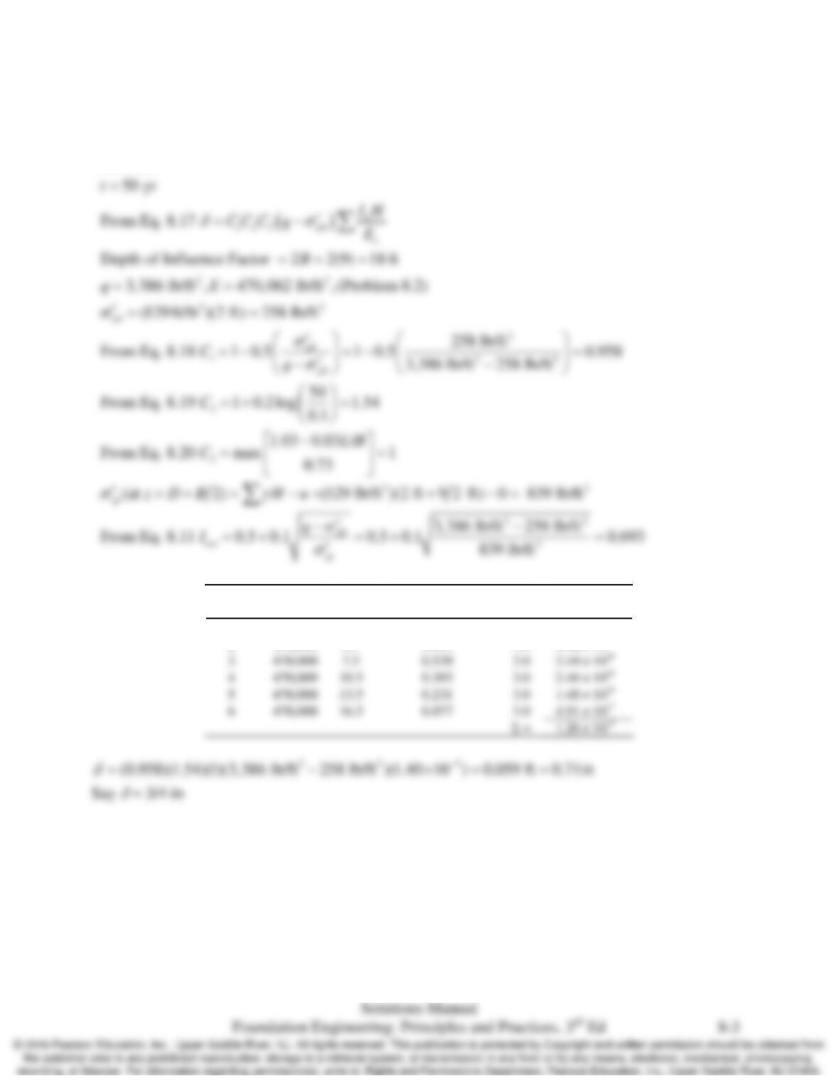
8.3 Repeat Problem 8.2 using Schmertmann’s method, compute the settlement of this footing at t = 50
yr.
Solution
Layer
No.
E
s
(lb/ft
2
)
z
f
(ft)
I
ε
Eqs. 8.12 & 8.13
H
(ft)
δ
Iε H/Es
1
470,000
1.5
0.298
3.0
1.90 × 10⁻⁶
2
470,000
4.5
0.693
3.0
4.42 × 10⁻⁶
3
470,000
7.5
0.539
3.0
4
470,000
0.385
3.0
5
470,000
0.231
3.0
6
470,000
0.077
Chap. 8 Spread Footings-Geotechnical Serviceability Limit States
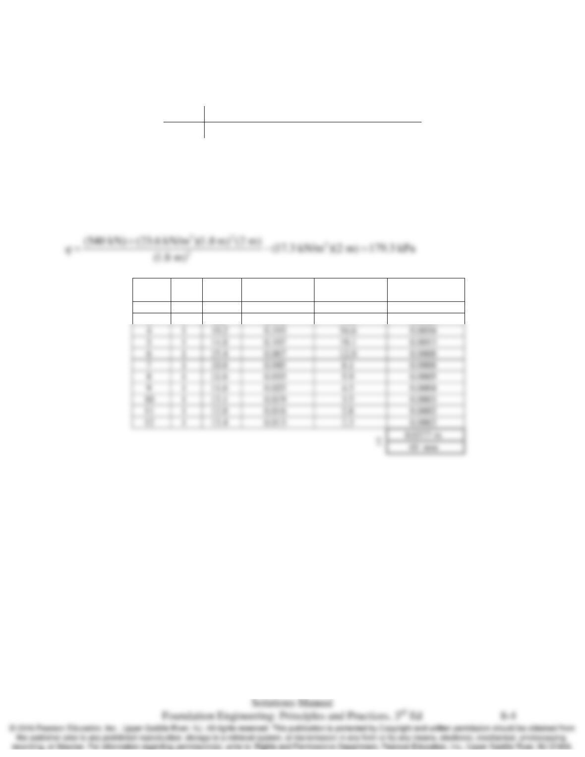
8.4 A 1.8 m square, 2 m deep footing supports a service load of 570 kN. It is supported on a clayey
sand. A dilatometer test run at the site has returned the following modulus profile.
Depth (m) 2 3 4 5 6 7 8 9 10 11 12
M (MPa) 7.7 8.8 10.2
14.8
15.4
10.8
11.6
11.6
13.1
13.8
13.4
Compute the footing settlement.
Solution
Assume unit weight of clayey sand = 17.3 kN/m3
Depth
(m)
H
(m)
M
(MPa)
I
q
From Eq. 3.14
Δσ
z
= q
ʹ
× I
q
(kPa)
δ = (Δσ
z
×H)/M
(m)
2
1
7.7
0.921
165.2
0.0215
3
1
8.8
0.418
74.9
0.0085
4
1
0.193
34.6
0.0034
5
1
0.107
19.1
0.0013
6
1
0.067
12.0
0.0008
7
1
0.045
0.0008
8
1
0.033
0.0005

Chap. 8 Spread Footings-Geotechnical Serviceability Limit States
8.5 Develop a spreadsheet to compute settlement of square footings using the incremental constrained
modulus method. The spreadsheet should allow input of: footing width, depth of footing, column
service load, and modulus as a function of depth. You will need to compute the stress distribution
of the applied stress using techniques discussed in Section 3.3 in order to compute the settlement.
Solution

Chap. 8 Spread Footings-Geotechnical Serviceability Limit States
8.6 Develop a spreadsheet to compute settlement of square footings using Schmertmann’s method.
The spreadsheet should allow input of: footing width, depth of footing, depth of water table, unit
weight of soil, column service load, and Es as a function of depth.
Solution
8.7 A 190-k column load is to be supported on a 10-ft square, 3-ft deep spread footing underlain by
young, normally consolidated sandy soils. The results of a representative CPT sounding at this
site are as follows:
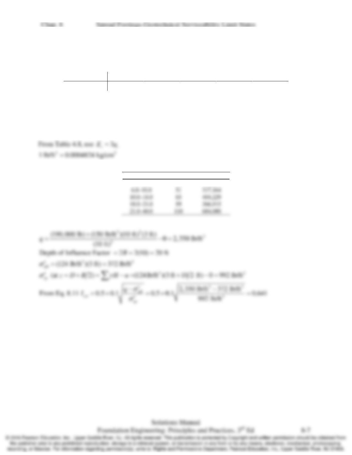
Depth (ft) 0.0–6.0 6.0–10.0 10.0–18.0 18.0–21.0 21.0–40.0
qc (kg/cm2) 30 51 65 59 110
The groundwater table is at a depth of 15 ft; the unit weight of the soil is 124 lb/ft3 above the
groundwater table and 130 lb/ft3 below. Using Schmertmann’s method, compute the total
settlement of this footing 30 years after construction.
Solution
51
317,164
65
404,229
59
366,915
684,080
Depth (ft)
qc (kg/cm2)
Es (lb/ft2)
0.0–6.0
30
186,567
Chap. 8 Spread Footings-Geotechnical Serviceability Limit States
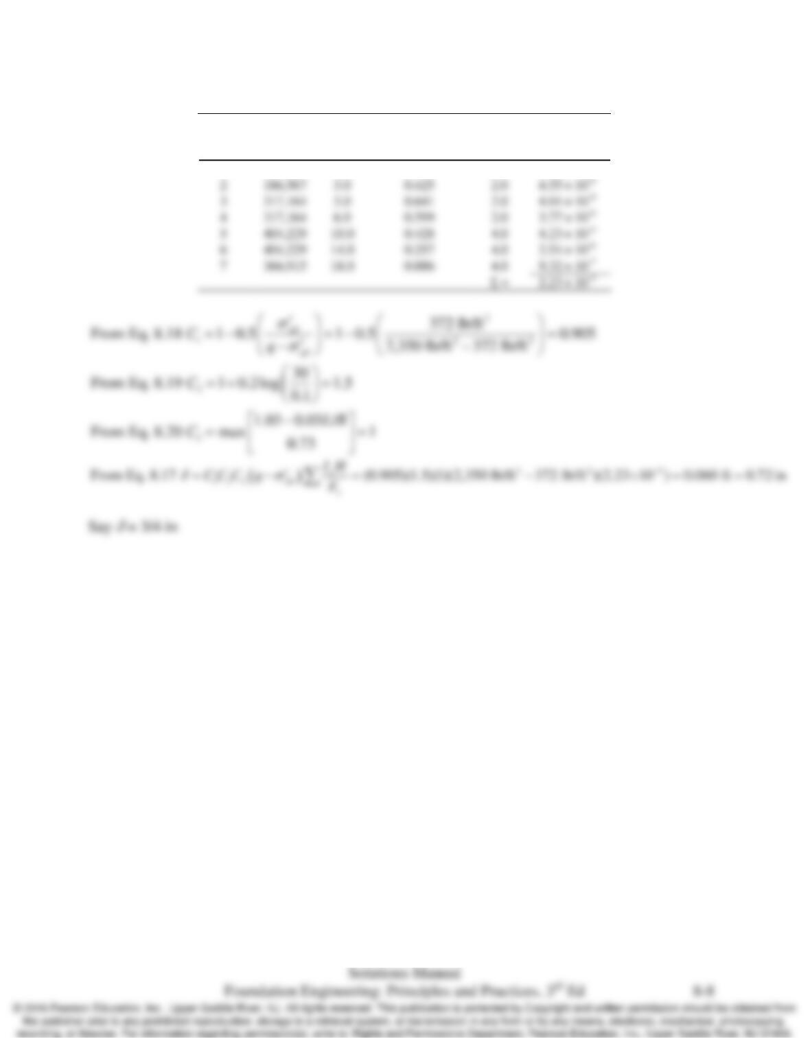
Layer
No.
Es
(lb/ft
2
)
zf
(ft)
Iε
Eqs. 8.14 & 8.15
H
(ft)
Iε H/Es
1
186,567
1.0
0.208
2.0
2.23 ×10⁻⁶
Chap. 8 Spread Footings-Geotechnical Serviceability Limit States
8.8 A 650-kN column load is supported on a 1.5-m wide by 2.0-m long by 0.5 m deep spread footing.
The soil below is a well graded, normally consolidated sand with γ = 18.0 kN/m3 and the
following SPT N60 values:
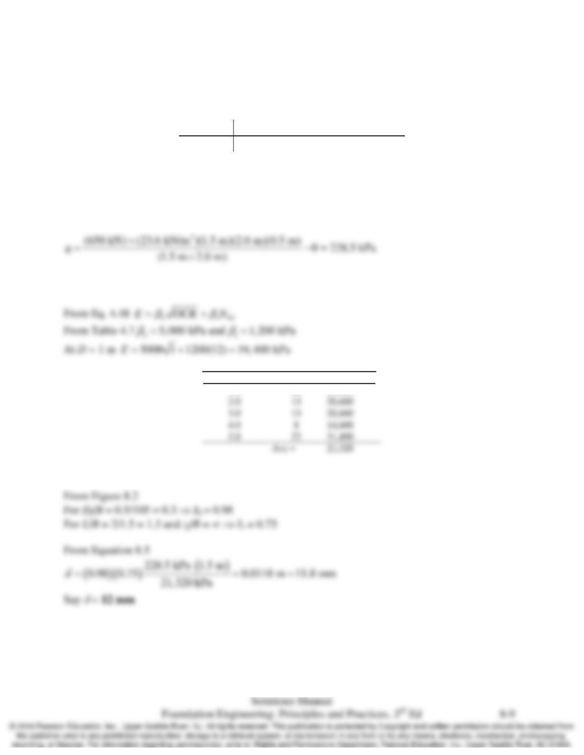
Depth (m)
1.0
2.0
3.0
4.0
5.0
N60
12
13
13
8
22
The groundwater table is at a depth of 25 m. Compute settlement of the footing using the
generalized elastic method with Christian and Carrier’s (1978) influence factors.
Solution
Normally consolidated, OCR = 1
2.0
13
20,600
Depth (m)
N60
E (kPa)
1.0
12
19,400
Chap. 8 Spread Footings-Geotechnical Serviceability Limit States
8.9 Repeat problem 8.8 using Schmertmann’s method, compute the total settlement at t = 30 yr
Solution
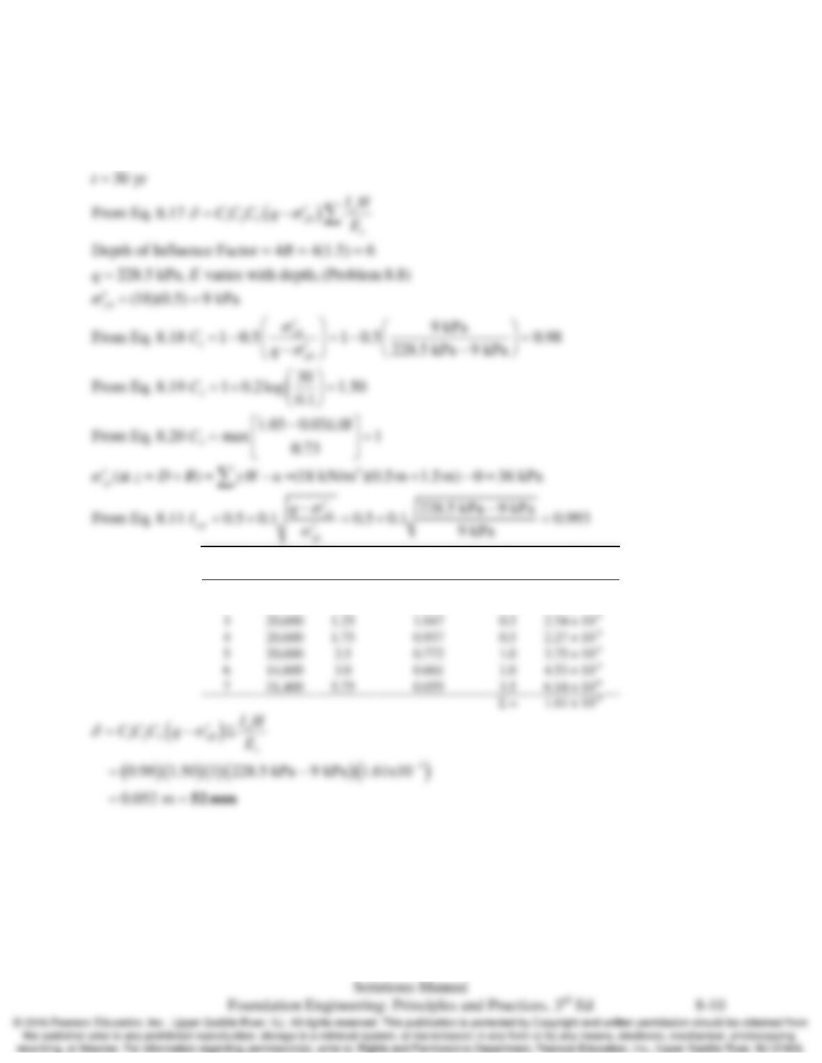
Layer
No.
E
s
(kPa)
z
f
(m)
I
ε
Eqs. 8.14 & 8.15
H
(m)
δ
Iε H/Es
1
19,400
0.25
0.332
0.5
8.56 ×10⁻⁶
2
19,400
0.75
0.597
0.5
1.54×10⁻⁵
3
20,600
1.25
1.047
0.5
2.54 ×10⁻⁵
4
20,600
1.75
0.937
0.5
5
20,600
0.772
1.0
3.75 ×10⁻⁵
6
14,600
0.661
1.0
4.53 ×10⁻⁵

Chap. 8 Spread Footings-Geotechnical Serviceability Limit States
8.10 A 300-k column load is to be supported on a 10-ft square, 4-ft deep spread footing. Cone
penetration tests have been conducted at this site, and the results are shown in Figure 8.8. The
groundwater table is at a depth of 6 ft, γ = 121 lb/ft3, and γsat = 125 lb/ft3 .
a. Compute the settlement of this footing using a spreadsheet.
b. The design engineer is considering the use of vibroflotation to densify the soils at this site (see
discussion in Chapter 26). This process would increase the qc values by 70 percent, and make the
soil slightly overconsolidated. The unit weights would increase by 5 lb/ft3. Use a spreadsheet to
compute the settlement of a footing built and loaded after densification by vibroflotation.
Solution
Chap. 8 Spread Footings-Geotechnical Serviceability Limit States
8.11 A proposed office building will include an 8-ft 6–in square, 3-ft deep spread footing that will
support a vertical downward service load of 160 k. The soil below this footing is an
overconsolidated clay (OC case I) with the following engineering properties: Cc/(1 + e0) = 0.10,
Cr/(1 + e0) = 0.022, and γ = 113 lb/ft3. This soil strata extends to a great depth and the
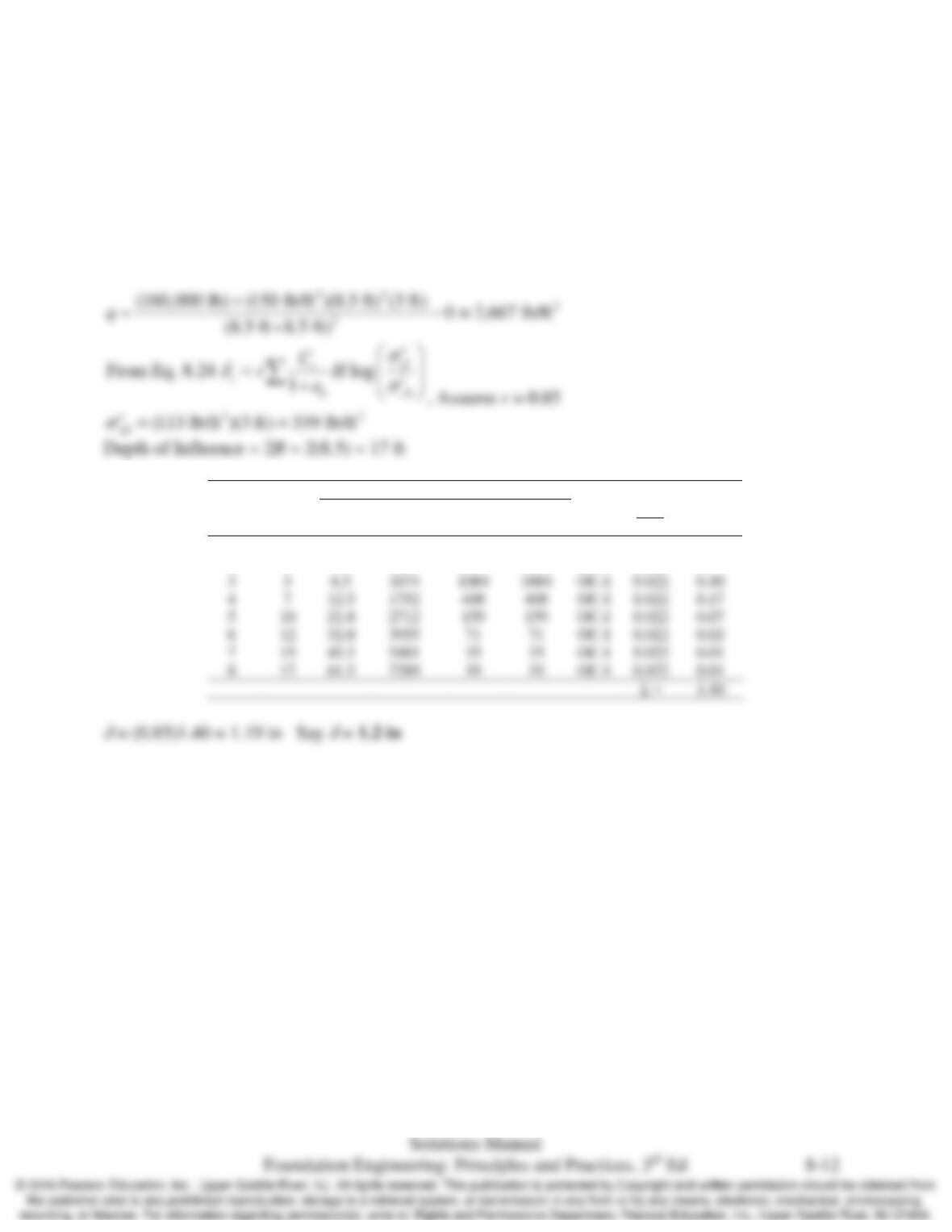
groundwater table is at a depth of 50 ft below the ground surface. Determine the total settlement
of this footing.
Solution
At midpoint of soil layer
Layer
No.
H
(ft)
zf (ft)
σ’
z0
(lb/ft
2
)
Δσ
z
(lb/ft
2
)
σ’
zf
(lb/ft
2
)
Case
0
1
r
C
e+
δ
c
(in)
1
1
0.5
396
2327
2722
OC-I
0.022
0.22
2
3
2.5
622
2115
2115
OC-I
0.022
0.51
3
5
6.5
1084
1084
OC-I
0.022
0.40
5
OC-I
0.022
0.07
6
OC-I
0.022
0.02
7
OC-I
0.022
0.01
8
OC-I
0.022
0.01
1.40