Section 8.1
Chapter 8
Section 8.1
8.1.1~e1,~e2is an orthonormal eigenbasis.
8.1.21
√21
1,1
√21
−1is an orthonormal eigenbasis.
8.1.5Eigenvalues −1, −1, 2
Choose ~v1=1
√2
−1
1
0
in E−1and ~v2=1
√3
1
1
1
in E2and let ~v3=~v1×~v2=1
√6
1
1
−2
.
8.1.61
3
2
2
1
,1
3
2
−1
−2
,1
3
1
−2
2
is an orthonormal eigenbasis.
8.1.91
√2
1
0
1
,1
√2
−1
0
1
,
0
1
0
is an orthonormal eigenbasis, with λ1= 3, λ2=−3, and λ3= 2, so
0
2
379
Chapter 8
8.1.11 1
√2
1
0
1
,1
√2
−1
0
1
,
0
1
0
is an orthonormal eigenbasis, with λ1= 2, λ2= 0, and λ3= 1, so S=
1
√2
1−1 0
0 0 √2
1 1 0
and D=
2 0 0
0 0 0
0 0 1
.
8.1.13 Yes; if ~v is an eigenvector of Awith eigenvalue λ, then ~v =I3~v =A2~v =λ2~v, so that λ2= 1 and λ= 1 or
λ=−1. Since Ais symmetric, E1and E−1will be orthogonal complements, so that Arepresents the reflection
about E1.
8.1.14 Let Sbe as in Example 3. Then S−1AS =
0 0 0
0 0 0
0 0 3
.
380
Section 8.1
8.1.15 Yes, if A~v =λ~v, then A−1~v =1
λ~v, so that an orthonormal eigenbasis for Ais also an orthonormal eigenbasis
for A−1(with reciprocal eigenvalues).
8.1.16 a ker(A) is four-dimensional, so that the eigenvalue 0 has multiplicity 4, and the remaining eigenvalue is
tr(A) = 5.
8.1.17 If Ais the n×nmatrix with all 1’s, then the eigenvalues of Aare 0 (with multiplicity n−1) and n. Now
B=qA + (p−q)In, so that the eigenvalues of Bare p−q(with multiplicity n−1) and qn +p−q. Thus
det(B) = (p−q)n−1(qn +p−q).
8.1.18 By Theorem 6.3.6, the volume is |det A|=pdet(ATA). Now ~vi·~vj=k~vikk~vjkcos(θ) = 1
2, so that ATAhas
8.1.19 Let L(~x) = A~x. Then ATAis symmetric, since (ATA)T=AT(AT)T=ATA, so that there is an orthonormal
8.1.20 By Exercise 19, there is an orthonormal basis ~v1, . . . , ~vmof Rmsuch that T(~v1),…,T(~vm) are orthogonal.
8.1.21 For each eigenvalue there are two unit eigenvectors: ±~v1,±~v2, and ±~v3. We have 6 choices for the first
column of S, 4 choices remaining for the second column, and 2 for the third.
8.1.22 a If we let k= 2 then Ais symmetric and therefore (orthogonally) diagonalizable.
b If we let k= 0 then 0 is the only eigenvalue (but A6= 0), so that Afails to be diagonalizable.
8.1.24 Note that Ais symmetric and orthogonal, so that the eigenvalues are 1 and −1 (see Exercise 23).
381
Chapter 8
8.1.25 Note that Ais symmetric an orthogonal, so that the eigenvalues of Aare 1 and −1.
1
0
0
1
0
0
1
0
0
1
8.1.26 Since Jnis both orthogonal and symmetric, the eigenvalues are 1 and −1. If nis even, then both have
multiplicity n
2(as in Exercise 24). If nis odd, then the multiplicities are n+1
2for 1 and n−1
2for −1 (as in
Exercise 25). One way to see this is to observe that tr(Jn) is 0 for even n, and 1 for odd n(recall that the trace
is the sum of the eigenvalues).
8.1.27 If nis even, then this matrix is Jn+In, for the Jnintroduced in Exercise 26, so that the eigenvalues are
2.
8.1.28 For λ6= 0
−λ0|1
|
−λ|1
|
...|.
.
−λ0|1
|
−λ|1
|
...|.
.
=−λ11(λ2−λ−12) = −λ11(λ−4)(λ+ 3)
Eigenvalues are 0 (with multiplicity 11), 4 and −3.
Eigenvalues for 0 are ~e1−~ei(i= 2,…,12),
382
Section 8.1
so
1111111111111
−1000000000011
0−1 0 0 0 0 0 0 0 0 0 1 1
0 0 −10000000011
0 0 0 −1 0 0 0 0 0 0 0 1 1
8.1.29 By Theorem 5.4.1 (im A)⊥= ker(AT) = ker(A), so that ~v is orthogonal to ~w.
8.1.30 The columns ~v, ~v2, . . . , ~vnof Rform an orthogonal eigenbasis for A=~v ~v T, with eigenvalues 1,0,0,…,0(n−
1 zeros), since
8.1.31 True; Ais diagonalizable, that is, Ais similar to a diagonal matrix D; then A2is similar to D2. Now
rank(D) = rank(D2) is the number of nonzero entries on the diagonal of D(and D2). Since similar matrices
have the same rank (by Theorem 7.3.6b) we can conclude that rank(A) = rank(D) = rank(D2) = rank(A2).
v1
383
Chapter 8
Algebraically, we can see this as follows: let A= [ ~v1~v2~v3], a 2 ×3 matrix.
3= 120◦.
8.1.34 Let ~v1, ~v2, ~v3, ~v4be such vectors. Form A= [ ~v1~v2~v3~v4], a 3 ×4 matrix.
Figure 8.2: for Problem 8.1.34.
The tips of ~v1, ~v2, ~v3, ~v4form a regular tetrahedron.
8.1.35 Let ~v1, . . . , ~vn+1 be these vectors. Form A= [ ~v1··· ~vn+1 ], an n×(n+ 1) matrix.
8.1.36 If ~v is an eigenvector with eigenvalue λ, then λ~v =A~v =A2~v =λ2~v, so that λ=λ2and therefore λ= 0
or λ= 1. Since Ais symmetric, E0and E1are orthogonal complements, so that Arepresents the orthogonal
projection onto E1.
Section 8.1
8.1.40 Using the terminology introduced in Exercise 8.1.39, we have
kA~uk=k−2c1~v1+ 3c2~v2+ 4c3~v3k=p4c2
1+ 9c2
2+ 16c2
2, which takes all values on the interval [2,4]. Geometri-
cally, the image of the unit sphere under Ais the ellipsoid with semi-axes 2, 3, and 4.
8.1.43 There is an orthonormal eigenbasis ~v1=1
√2
1
−1
0
, ~v2=1
√6
1
1
−2
, ~v3=1
√3
1
1
1
with associated
1
8.1.44 Use Exercise 8.1.43 as a guide. Consider an orthonormal eigenbasis ~v1, …., ~vnfor A, with associated eigen-
values λ1≤λ2≤…. ≤λn, listed in ascending order. If ~v =c1~v1+… +cn~vnis any nonzero vector in Rn, then
8.1.45 a If S−1AS is upper triangular then the first column of Sis an eigenvector of A. Therefore, any matrix
without real eigenvectors fails to be triangulizable over R, for example, 0−1
1 0 .
8.1.46 a By definition of an upper triangular matrix, ~e1is in ker U,~e2is in ker(U2), . . . , ~enis in ker(Un), so that all
~x in Cnare in ker(Un), that is, Un= 0.
Chapter 8
8.1.47 a For all i, j, “n
X
k=1
aikbkj #≤
n
X
k=1 |aikbkj |=
n
X
k=1 |aik||bkj |
↑
triangle inequality
8.1.49 Let λbe the largest |rii|; note that λ < 1. Then |R|=
|r11| ∗
...
0|rnn|
≤
λ∗
...
0λ
=λ
1∗
...
0 1
=
λ(In+U), and |Rt| ≤ |R|t≤λt(In+U)t≤λttn(In+U+···+Un−1).
Section 8.2
8.2.1We have a11 = coefficient of x2
1= 6, a22 = coefficient of x2
2= 8, a12 =a21 =1
2( coefficient of x1x2) = −7
2.
So, A=6−7
2
−7
28
386
Section 8.2
8.2.4A=6 2
2 3 , positive definite
8.2.8If S−1AS =Dis diagonal, then S−1A2S=D2, so that all eigenvalues of A2are ≥0. So A2is positive
semi-definite; it is positive definite if and only if Ais invertible.
8.2.9a (A2)T= (AT)2= (−A)2=A2, so that A2is symmetric.
8.2.10 L(~x)=(~x+~v)TA(~x +~v)−~xTA~x −~v TA~v =~x TA~x +~x TA~v +~v TA~x +~v TA~v −~xTA~x −~v TA~v =~xTA~v +~v TA~x =
~v TA~x +~v TA~x = (2~v TA)~x,
8.2.11 The eigenvalues of A−1are the reciprocals of those of A, so that Aand A−1have the same definiteness.
8.2.13 q(~ei) = ~ei·A~ei=aii >0
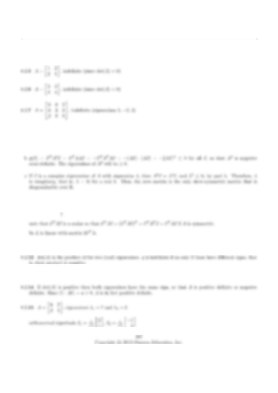
1,~v2=1
2
Chapter 8
λ1c2
1+λ2c2
2= 1 or 7c2
1+ 2c2
2= 1.(See Figure 8.3.)
v2
E7
Figure 8.3: for Problem 8.2.15.
8.2.16 A=01
2
1
2, and λ2=−1
2
8.2.17 A=3 2
2 0 , eigenvalues λ1= 4, λ2=−1
8.2.18 A=9−2
−2 6 , eigenvalues λ1= 10, λ2= 5
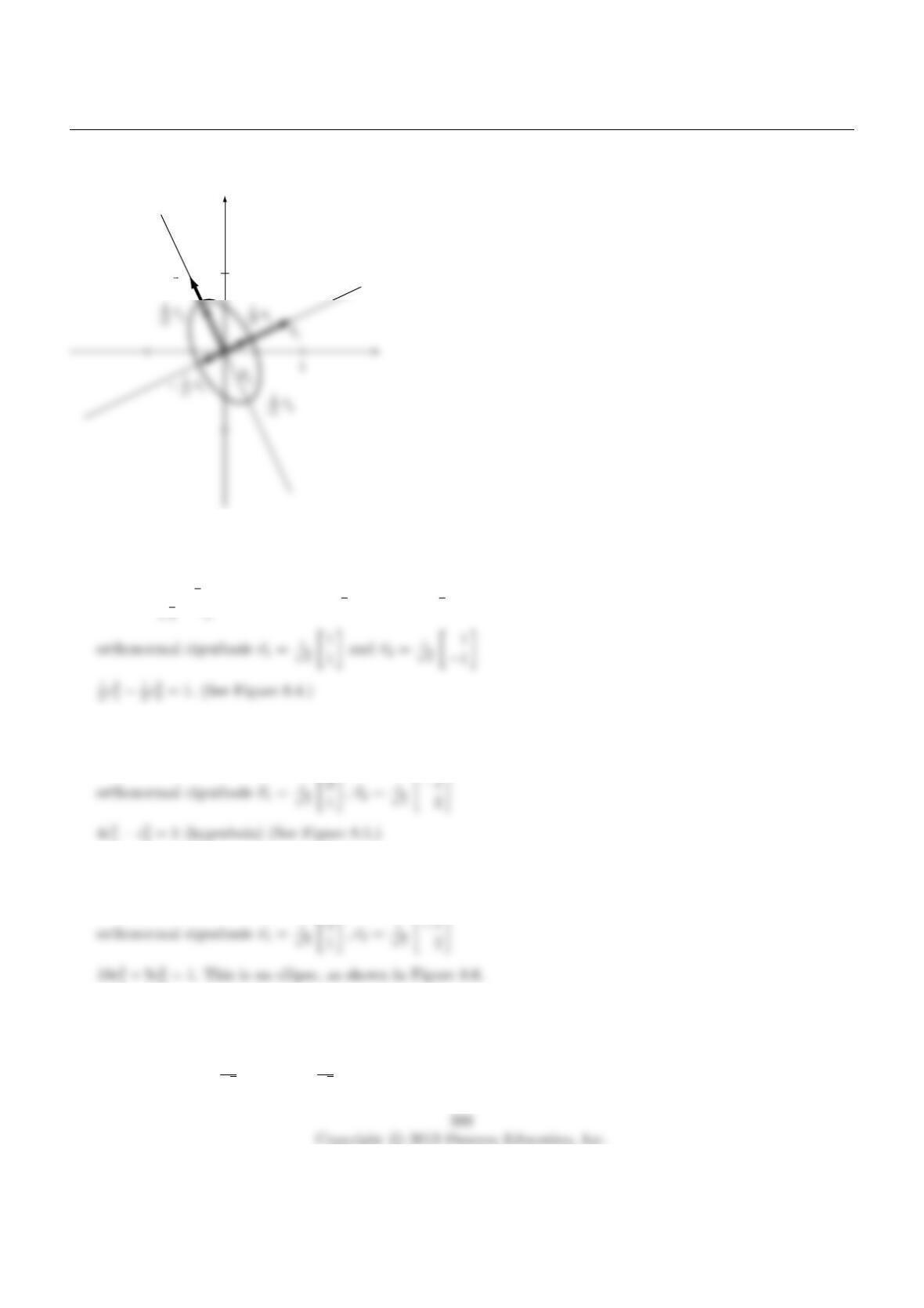
8.2.19 A=1 2
2 4 ; eigenvalues λ1= 5, λ2= 0
eigenvectors ~v1=1
√51
2,~v2=1
√5−2
1
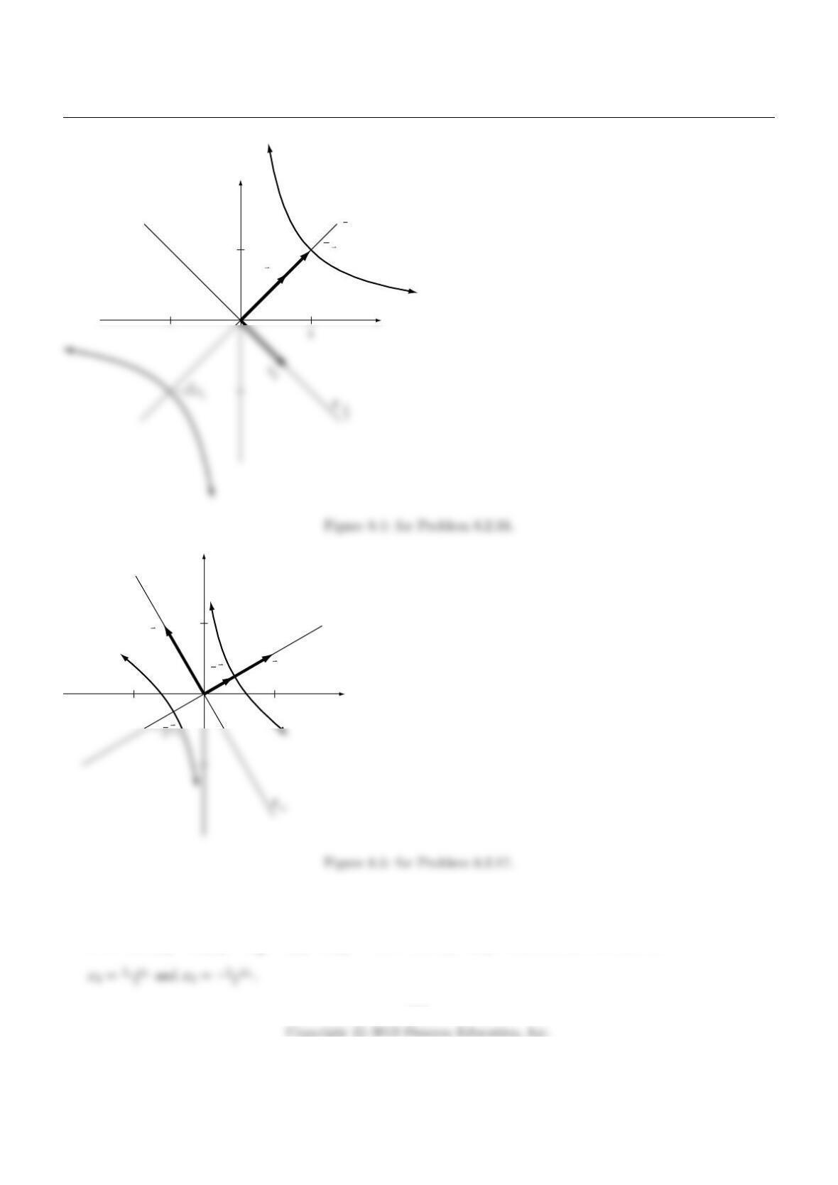
Section 8.2
√2v1
v1
1
2
E
v1
v2
E4
1
1
v1
1
2
5c2
1= 1 (a pair of lines) (See Figure 8.7.)
Note that (x2
1+ 4x1x2+ 4x2
2) = (x1+ 2x2)2= 1, so that x1+ 2x2=±1, and the two lines are
389
Chapter 8
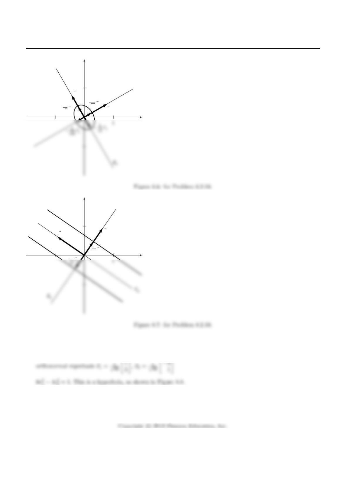
v1
v2
E10
1v2
√5
1v1
√10
v2
1v1
√5
1v1
v1
8.2.20 A=−3 3
3 5 ; eigenvalues λ1= 6 and λ2=−4
8.2.21 a In each case, it is informative to think about the intersections with the three coordinate planes: x1−x2,
x1−x3, and x2−x3.
390
Section 8.2
v2
1v1
v1
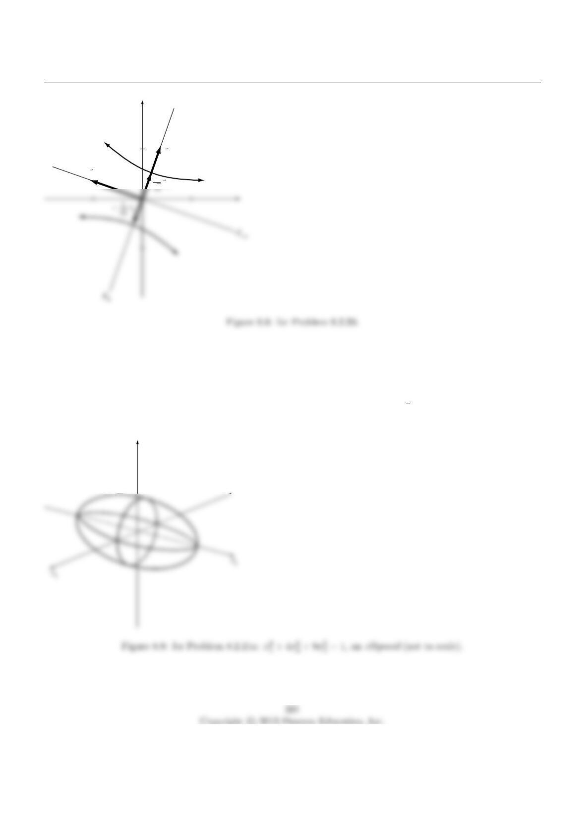
•] For the surface x2
1+ 4x2
2+ 9x2
3= 1, all these intersections are ellipses, and the surface itself is an ellipsoid .
This surface is connected and bounded; the points closest to the origin are ±
0
0
1
3
, and those farthest ±
1
0
0
.
(See Figure 8.9.)
x3
•] In the case of x2
1+ 4x2
2−9x2
3= 1, the intersection with the x1−x2plane is an ellipse, and the two other
intersections are hyperbolas. The surface is connected and not bounded; the points closest to the origin are
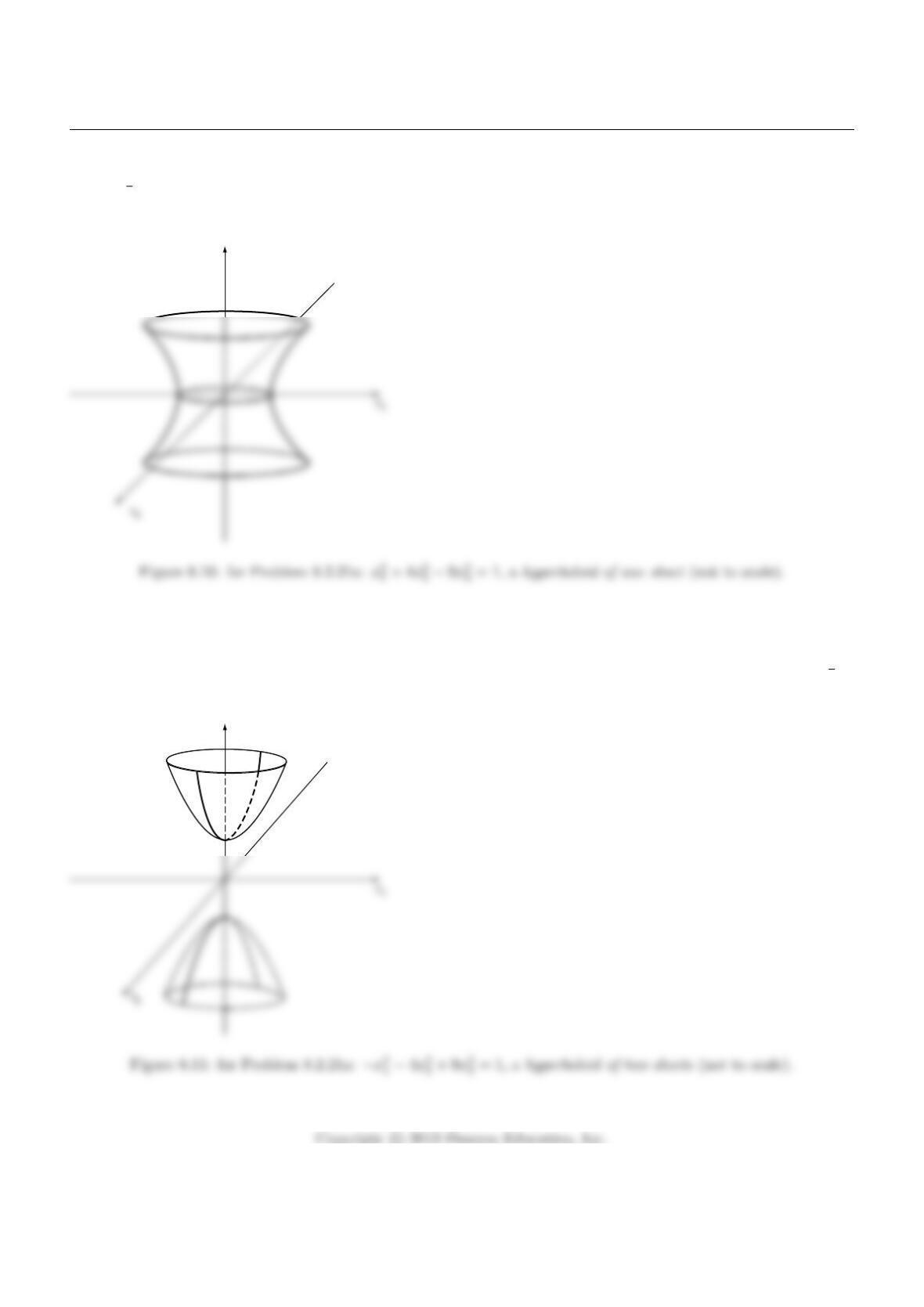
Chapter 8
±
0
1
2
0
. (See Figure 8.10.)
x3
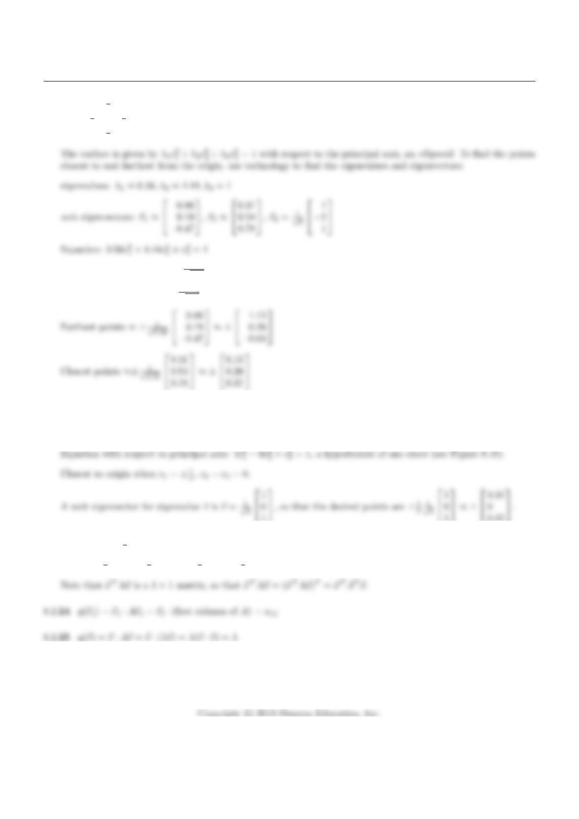
•] In the case −x2
1−4x2
2+9x2
3= 1, the intersection with the x1−x2plane is empty, and the two other intersections
are hyperbolas. The surface consists of two pieces and is unbounded. The points closest to the origin are ±
0
0
1
3
.
(See Figure 8.11.)
x3
392
Section 8.2
bA=
11
21
1
223
2
13
23
is positive definite, with three positive eigenvalues λ1, λ2, λ3.
Farthest points when c1=±1
√0.56 and c2=c3= 0
Closest points when c2=±1
√4.44 and c1=c3= 0
8.2.22 A=
−1 0 5
0 1 0
5 0 −1
; eigenvalues λ1= 4, λ2=−6, λ3= 1
8.2.23 Yes; M=1
2(A+AT) is symmetric, and
~xTM~x =1
2~xTA~x +1
2~xTAT~x =1
2~xTA~x +1
2~xTA~x =~x TA~x
↑
~v is a unit vector
393
Chapter 8
8.2.26 False; If A=0 1
1 0 then q1
0=1
0·0 1
1 0 1
0=1
0·0
1= 0.
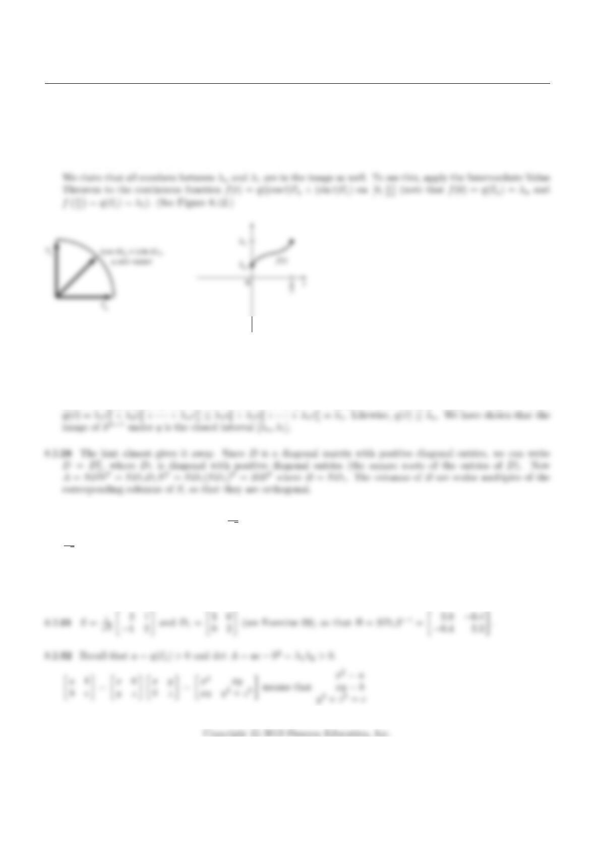
8.2.27 Let ~v1, . . . , ~vnbe an orthonormal eigenbasis for Awith A~vi=λi~vi. We know that q(~vi) = λi(see Exercise 25),
so that q(~v1) = λ1and q(~vn) = λnare in the image.
Figure 8.12: for Problem 8.2.27.
The Intermediate Value Theorem tells us that for any cbetween λnand λ1, there is a t0such that f(t0) =
q((cos t0)~vn+ (sin t0)~v1) = c. Note that (cos t0)~vn+ (sin t0)~v1is a unit vector. Now we will show that, conversely,
q(~v) is on [λn, λ1] for all unit vectors ~v. Write ~v =c1~v1+···+cn~vnand note that k~vk2=c2
1+···+c2
n= 1. Then
8.2.29 From Example 1 we have S=1
√52 1
−1 2 and D=9 0
0 4 . Let D1=3 0
0 2 and B=SD1=
1
√56 2
−3 4 .
8.2.30 Define D1as in Exercise 28. Then A=SDS−1=SD1D1S−1= (SD1S−1)(SD1S−1) = B2, where B=
SD1S−1.Bis positive definite, since S−1BS =D1is diagonal with positive diagonal entries.
394