20. a. Correlations: ChickConsum, Income, ChickPrice, PorkPrice, BeefPrice
ChickConsum Income ChickPrice PorkPrice
LnChickC LnIncome LnChickP LnPorkP
LnIncome 0.952
b. Stepwise Regression: ChickConsum versus Income, ChickPrice, …
Response is ChickConsum on 4 predictors, with N = 23
Step 1 2
ChickPrice -0.29
c. There is high multicollinearity among the predictor variables so the final model
depends on which non-significant predictor variable is deleted first. If BeefPrice is
The regression equation is
Analysis of Variance
21. Stepwise Regression: LnChickC versus LnIncome, LnChickP, …
Response is LnChickC on 4 predictors, with N = 23
Step 1 2
S 0.0528 0.0321
161
Final model is the one selected by stepwise regression. There is no significant
residual autocorrelation.
The regression equation is
Analysis of Variance
Source DF SS MS F P
Regression 2 0.61001 0.30500 295.30 0.000
The coefficient of .44 on LnIncome implies as Income increases 1% chicken
22. The regression equation is
22 cases used, 1 cases contain missing values
Predictor Coef SE Coef T P VIF
162
Source DF SS MS F P
Regression 2 8.039 4.020 2.72 0.091
Very little explanatory power in the predictor variables. If the non-significant DiffIncome
23. The regression equation is
22 cases used, 1 cases contain missing values
Predictor Coef SE Coef T P
Analysis of Variance
Source DF SS MS F P
Regression 1 769.45 769.45 432.71 0.000
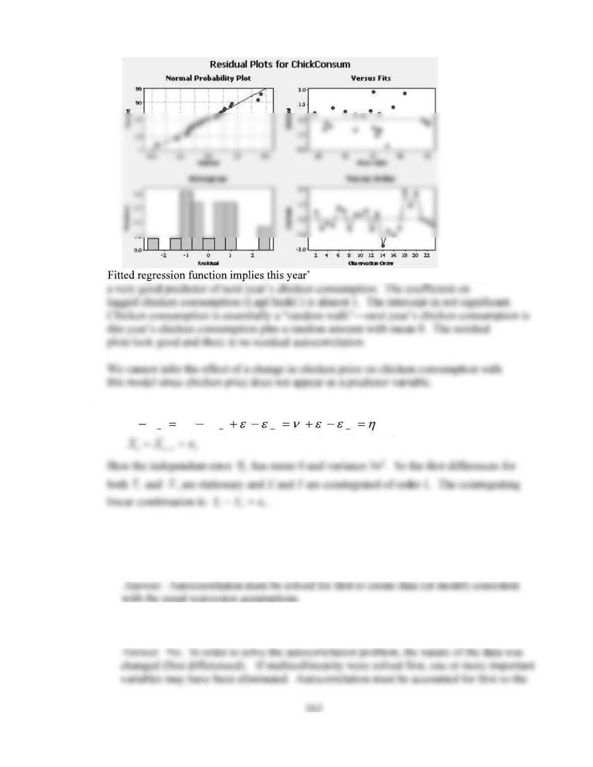
s chicken consumption is likely to be
24.
tttttttttt
XXYY
1111
say
CASE 8-2: BUSINESS ACTIVITY INDEX FOR SPOKANE COUNTY
1. Why did Young choose to solve the autocorrelation problem first?
2. Would it have been better to eliminate multicollinearity first and then tackle
autocorrelation?

3. How does the small sample size affect the analysis?
4. Should the regression done on the first differences have been through the origin?
5. Is there any potential for the use of lagged data?
6. What conclusions can be drawn from a comparison of the Spokane County business
activity index and the GNP?
CASE 8-3: RESTAURANT SALES
1.
2. Was it correct to use lagged sales as a predictor variable?
3.
4. Would another type of forecasting model be more effective for forecasting weekly sales?
165
CASE 8-4: MR. TUX
John is correct to be disappointed with the model run with seasonal dummy variables since
CASE 8-5: CONSUMER CREDIT COUNSELING
Nonseasonal model:
The regression equation is
Predictor Coef SE Coef T P
Constant -292.27 41.23 -7.09 0.000
Analysis of Variance
Source DF SS MS F P
Regression 3 34630 11543 41.62 0.000
The best nonseasonal regression model used the business activity index, number of
bankruptcies filed, and number of building permits to forecast number of clients seen. The
Durbin-Watson test for serial correlation is inconclusive at the .05 level. The residual
autocorrelation function shows some significant autocorrelation around lag 4.
Best seasonal model:
The regression equation is
166
Predictor Coef SE Coef T P
Constant -135.08 26.96 -5.01 0.000
Index 2.5099 0.2421 10.37 0.000
S4 -15.869 8.445 -1.88 0.064
S5 -21.146 8.441 -2.51 0.015
Analysis of Variance
Source DF SS MS F P
The best seasonal model uses Index and 11 seasonal dummy variables to represent
the months Feb through Dec. We retain all the seasonal dummy variables for forecasting
purposes even though some are non-significant. The Durbin-Watson test is inconclusive at the
.05 level. The residual autocorrelations have a just significant spike at lag 6 but are otherwise
non-significant. Forecasts for the first three months of 1993 follow.
Forecast Actual
Jan 1993 179 151
Autoregressive model:
Autoregressive models with number of new clients lagged 1, 4 and 12 months were
tried. None of these models proved to be useful for forecasting. The best model had number of
167
The regression equation is
95 cases used, 1 cases contain missing values
Predictor Coef SE Coef T P
Analysis of Variance
Source DF SS MS F P
CASE 8-6: AAA WASHINGTON
1. The results for the best model are shown below (see also solution to Case 7-2). Each of
the independent variables is significantly different from 0 at the .05 level. The signs of
the coefficients are what we would expect them to be.
The regression equation is
Predictor Coef SE Coef T P
Constant 17060.2 847.0 20.14 0.000
Analysis of Variance
Source DF SS MS F P
168
2. Serial correlation is not a problem. The value of the Durbin-Watson statistic (1.62)
CASE 8-7 ALOMEGA FOOD STORES
1. Julie appears to have a good regression equation with an R-squared of 91%.
Additional significant explanatory variables may be available but there is not much
2.
Tilson, ties the statistical exercise in the Alomega case to the real world of business
3. As noted in the case, the advertising predictor variables are under the control of
Alomega management. Students can demonstrate the usefulness of this result by
that is identical to the past except for the identified predictor variables. If her
169
CASE 8-8 SURTIDO COOKIES
2. in cookie sales is explained
3. Forecasts:
June 2003 733,122
4. The regression equation is
29 cases used, 12 cases contain missing values
Analysis of Variance
Source DF SS MS F P
This regression model is very reasonable. About 81% of the variation in cookie
Forecasts:
June 2003 717,956
July 2003 632,126
5. Both models fit the data well. Apart from July 2003, the forecasts generated by the
CASE 8-9 SOUTHWEST MEDICAL CENTER
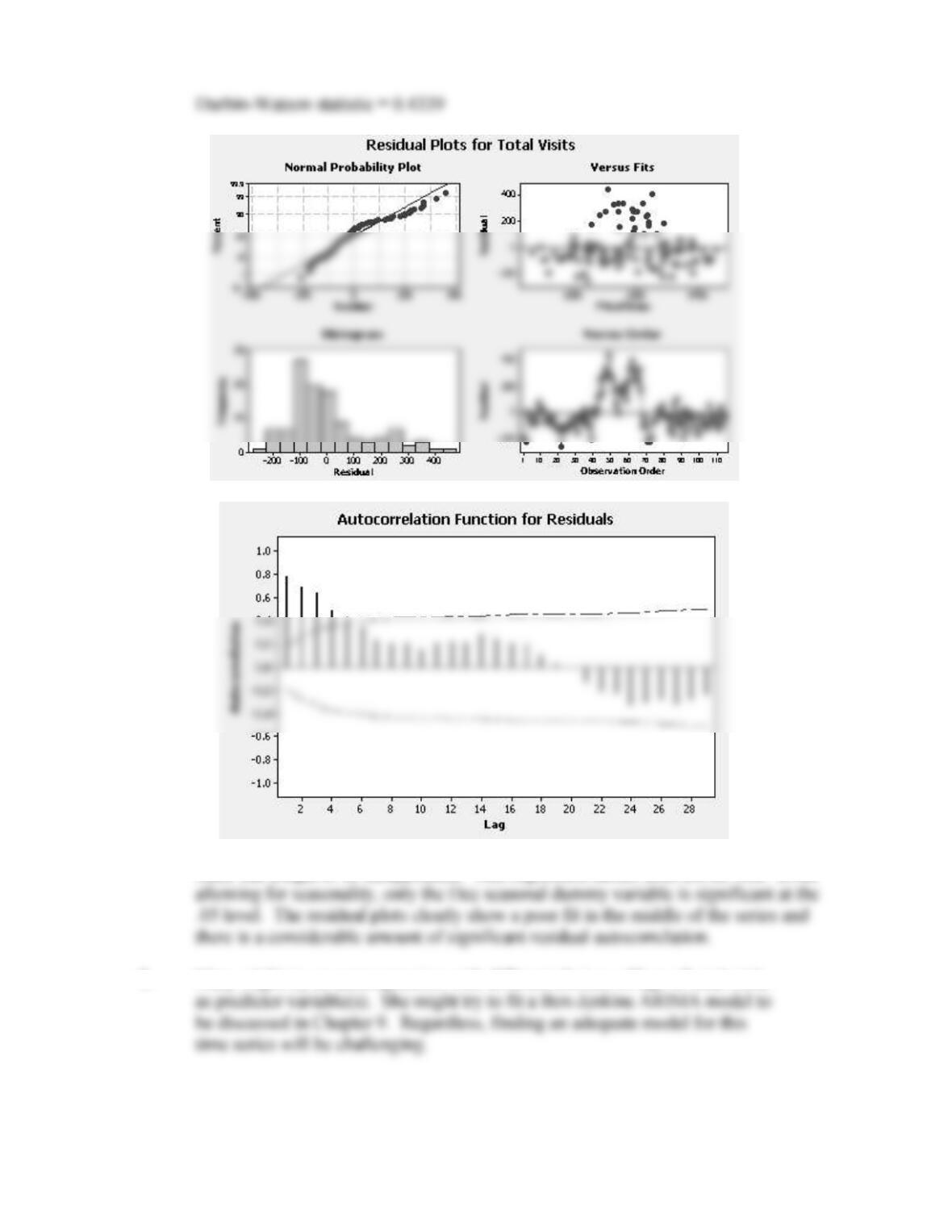
1. The regression results along with residual plots and the residual autocorrelation
function follow.
The regression equation is
Predictor Coef SE Coef T P
Constant 996.97 58.42 17.06 0.000
Nov -118.34 71.66 -1.65 0.102
Mar 23.80 73.55 0.32 0.747
Analysis of Variance
Source DF SS MS F P
171
Mary has a right to be disappointed. This regression model does not fit well. Even
2. Mary might try an autoregression with different choices of lags of total visits