146
CHAPTER 8
REGRESSION WITH TIME SERIES DATA
ANSWERS TO PROBLEMS AND CASES
1. If not properly accounted for, serial correlation can lead to false inferences under the
usual regression assumptions. Regressions can be judged significant when, in fact,
2. Serial correlation often arises naturally in time series data. Series, like employment,
whose magnitudes are naturally related to the seasons of the year will be autocorrelated.
7. Serial correlation can be eliminated by specification of the regression function (using
the best predictor variables) consistent with the usual regression assumptions. This can
8. A predictor variable is generated by using the Y variable lagged one or more periods.
9. The regression equation is
147
Analysis of Variance
Source DF SS MS F P
The null and alternative hypotheses are:
10. The regression equation is
Predictor Coef SE Coef T P
Constant 309899 59496 5.21 0.000
Analysis of Variance
Source DF SS MS F P
correlation.
11. Serial correlation is not a problem. However, it is interesting to see whether the students
realize that collinearity is a likely problem since Customer and Charge are highly correlated.
Correlation matrix:
Revenue Use Charge
148
The regression equation is
Analysis of Variance
The regression equation is
Analysis of Variance
Source DF SS MS F P
12. a. Correlations: Share, Earnings, Dividend, Payout
Share Earnings Dividend
149
Earnings 0.565
The best model, after taking account of the initial multicollinearity, uses the predictor
variables Earnings and Payout (ratio).
The regression equation is
Analysis of Variance
Source DF SS MS F P
13. a.
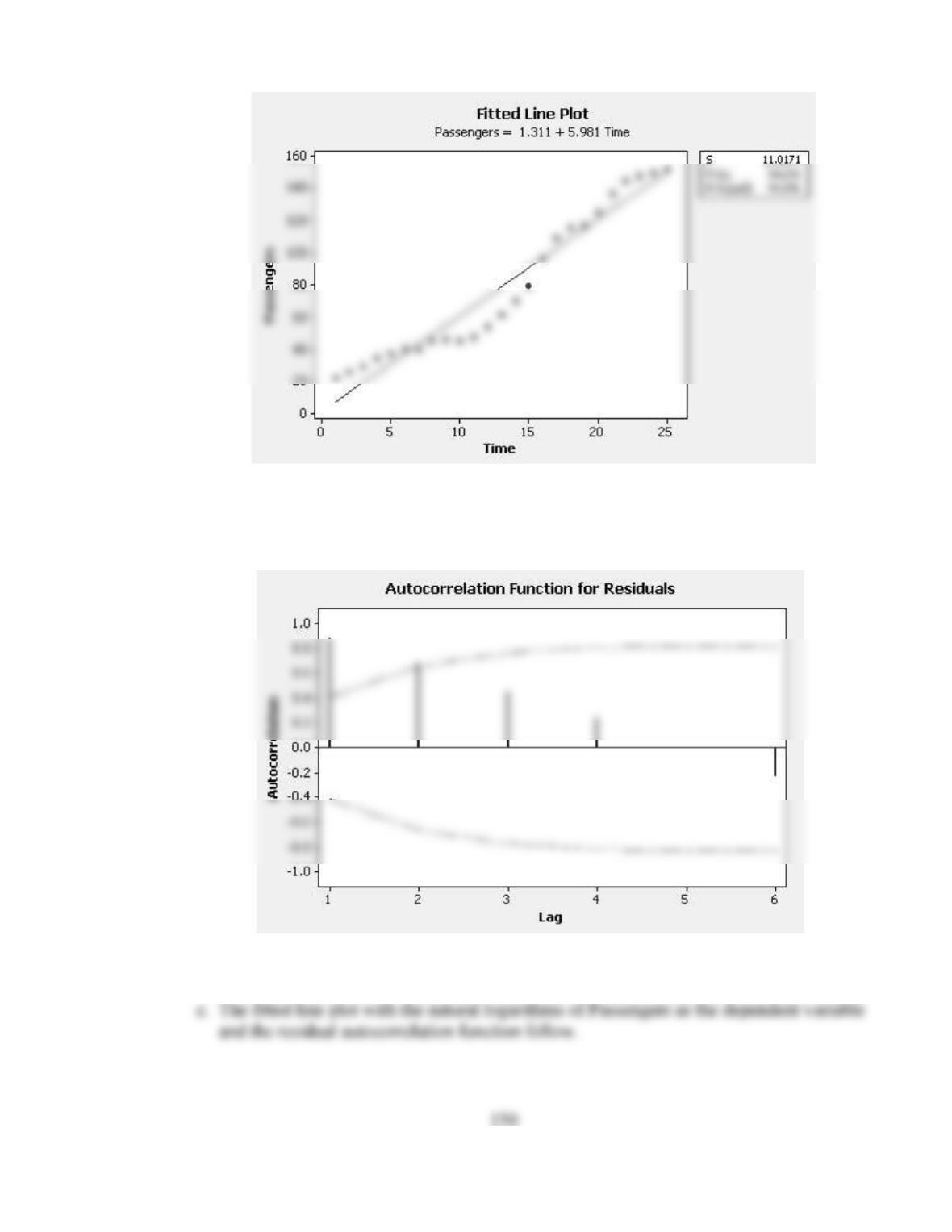
b. No. The residual autocorrelation function for the residuals from the straight line fit
indicates significant positive autocorrelation. The independent errors assumption
is not viable.
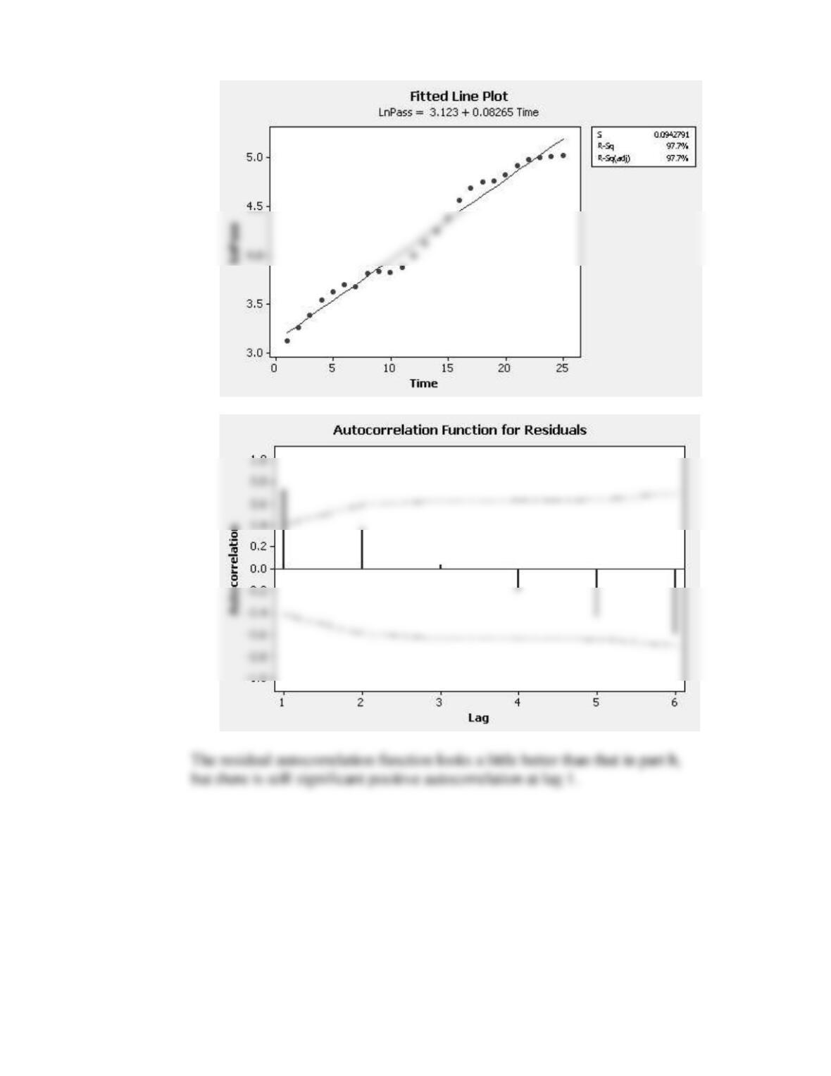
151
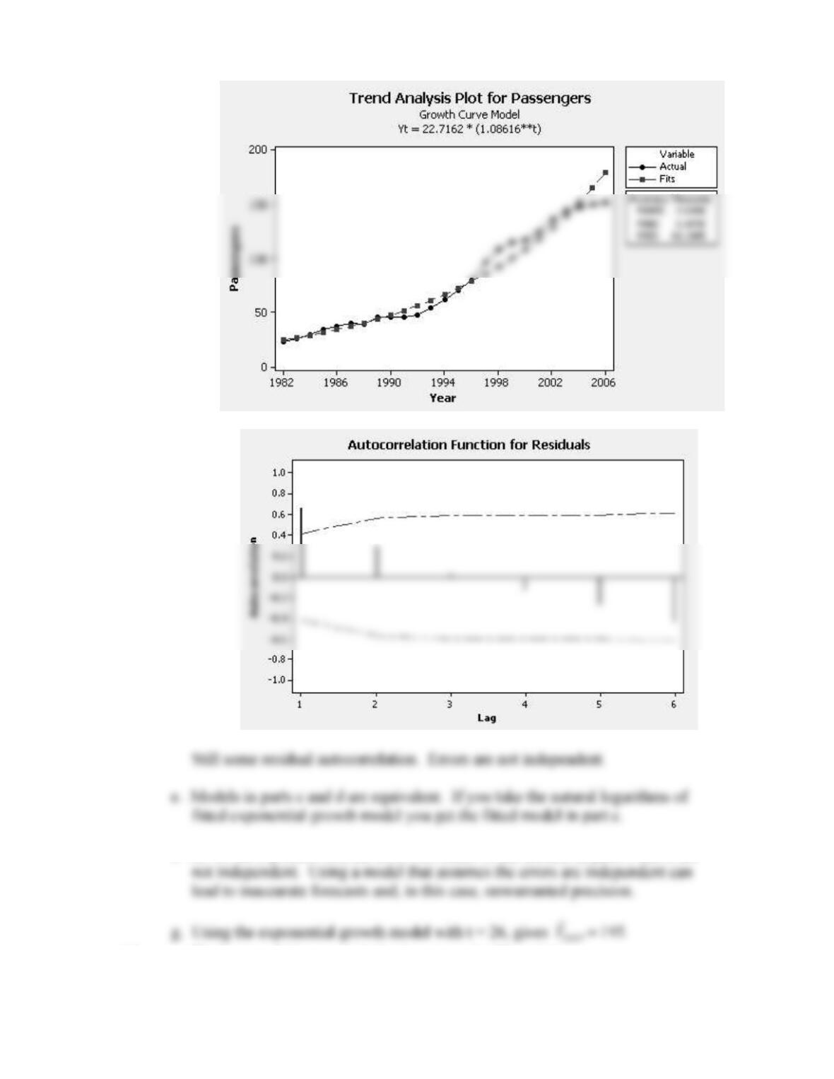
d. Exponential trend plot for Passengers follows along with residual autocorrelation
function.
152
f. As we have pointed out, the errors for either of the models in parts c and d are
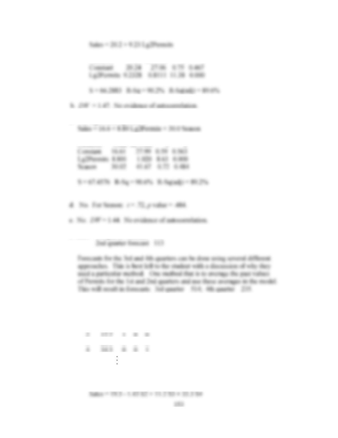
14. a. The best model lags permits by 2 quarters (Lg2Permits):
Predictor Coef SE Coef T P
c. The regression equation is
Predictor Coef SE Coef T P
f. 2007 1st quarter forecast 177
15.
Quarter Sales S2 S3 S4
1 16.3 0 0 0
3 28.1 0 1 0
4 34.3 0 0 1
The regression equation is
154
Predictor Coef SE Coef T P
Analysis of Variance
Source DF SS MS F P
Regression 3 8726.5 2908.8 56.36 0.000
16. a. & b. The regression equation is
Predictor Coef SE Coef T P
155
c. 585. . Calculate the generalized differences
1
‘
585.
ttt
YYY
and
d. The standard error of
1
is smaller in the initial regression than it is in the
17. The regression equation is
20 cases used, 1 cases contain missing values
Predictor Coef SE Coef T P
Analysis of Variance
Source DF SS MS F P
1
1
18. a. The regression equation is
Savings = 4.98 + 0.0577 Income
Analysis of Variance
Source DF SS MS F P
b. The regression equation is
Analysis of Variance
Source DF SS MS F P
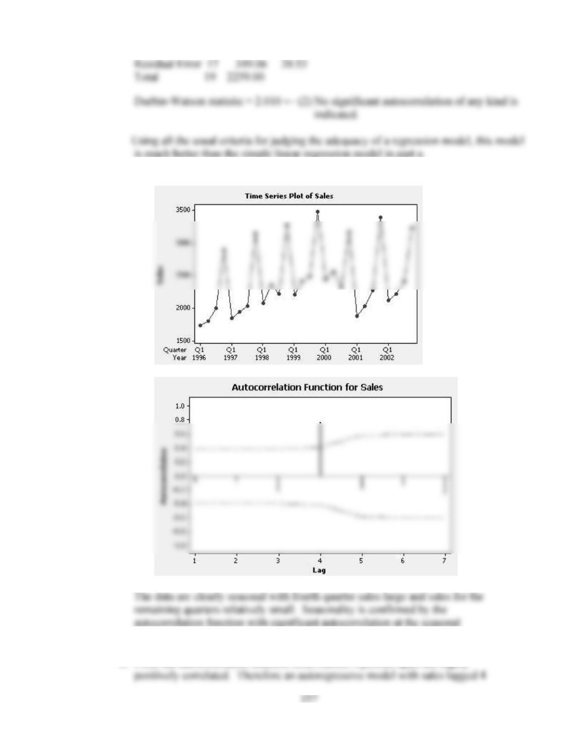
19. a.
lag 4.
b. From the autocorrelation function observations 4 periods apart are highly
158
c. The regression equation is
Predictor Coef SE Coef T P
Analysis of Variance
Source DF SS MS F P
Total 23 6011528
d. May 31 (2003)
Y
= 421.4 + .85273(2118) = 2227.5 compared to 2150