144
Chapter 8
of Taxation
WHAT’S NEW IN THE SIXTH EDITION:
A new
In the News
box on “New Research on Taxation” has been added.
LEARNING OBJECTIVES:
By the end of this chapter, students should understand:
➢ how taxes reduce consumer and producer surplus.
CONTEXT AND PURPOSE:
Chapter 8 is the second chapter in a three-chapter sequence dealing with welfare economics. In the
previous section on supply and demand, Chapter 6 introduced taxes and demonstrated how a tax affects
the price and quantity sold in a market. Chapter 6 also described the factors that determine how the
burden of the tax is divided between the buyers and sellers in a market. Chapter 7 developed welfare
economics—the study of how the allocation of resources affects economic well-being. Chapter 8
8
APPLICATION: THE COSTS OF
TAXATION
Chapter 8 /Application: The Costs of Taxation ❖ 145
KEY POINTS:
• A tax on a good reduces the welfare of buyers and sellers of the good, and the reduction in
consumer and producer surplus usually exceeds the revenue raised by the government. The fall in
total surplus—the sum of consumer surplus, producer surplus, and tax revenue—is called the
deadweight loss of the tax.
CHAPTER OUTLINE:
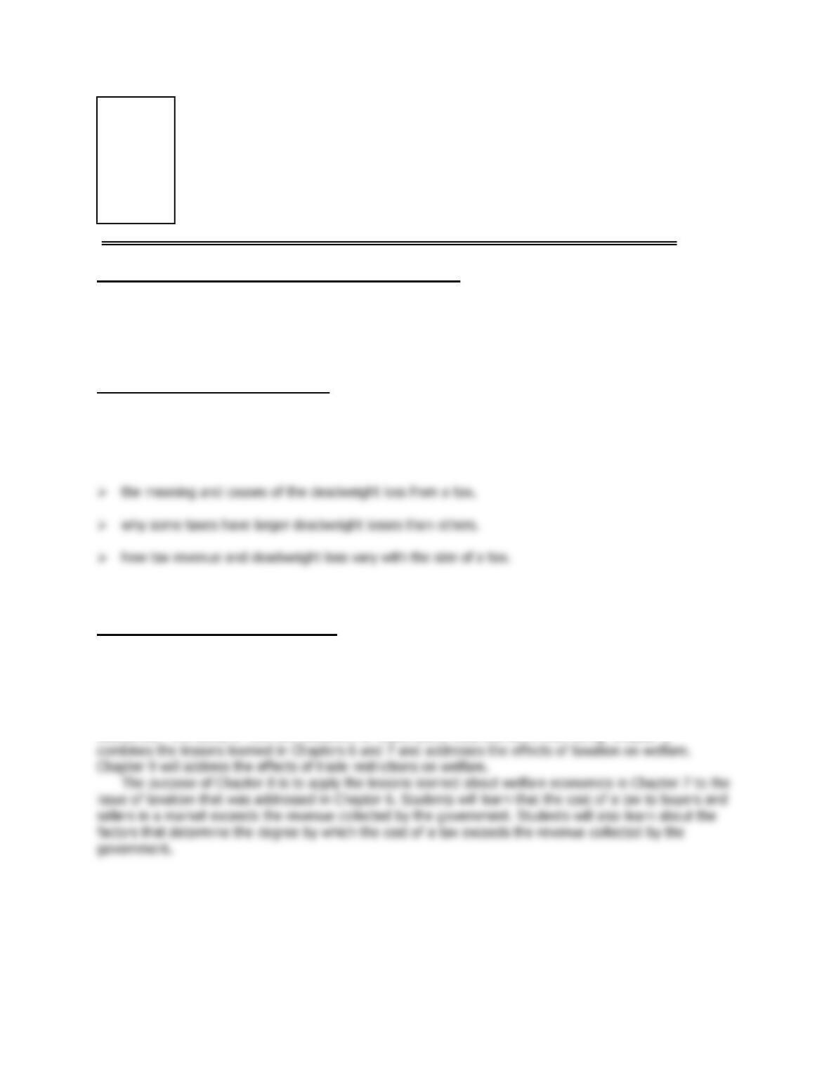
I. The Deadweight Loss of Taxation
A. Remember that it does not matter who a tax is levied on; buyers and sellers will likely share in
the burden of the tax.
Figure 1
146 ❖ Chapter 8 /Application: The Costs of Taxation
C. How a Tax Affects Market Participants
1. We can measure the effects of a tax on consumers by examining the change in consumer
surplus. Similarly, we can measure the effects of the tax on producers by looking at the
change in producer surplus.
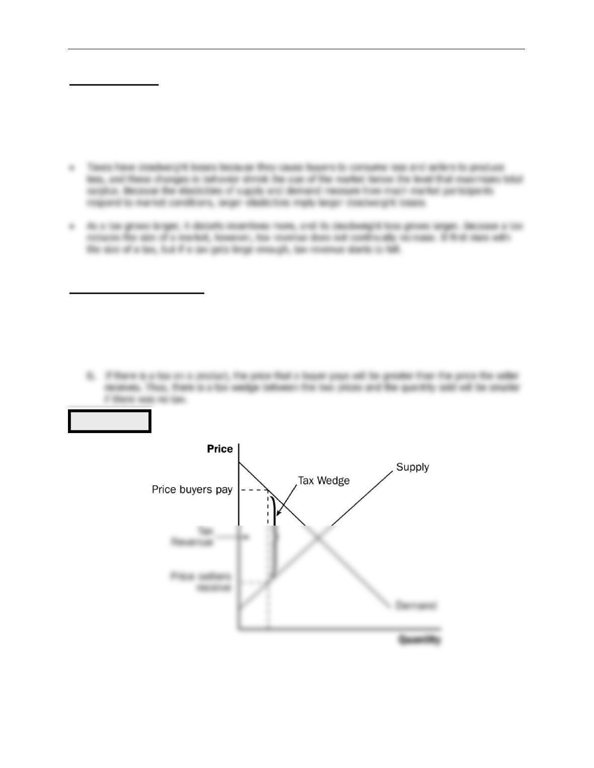
3. Welfare without a Tax
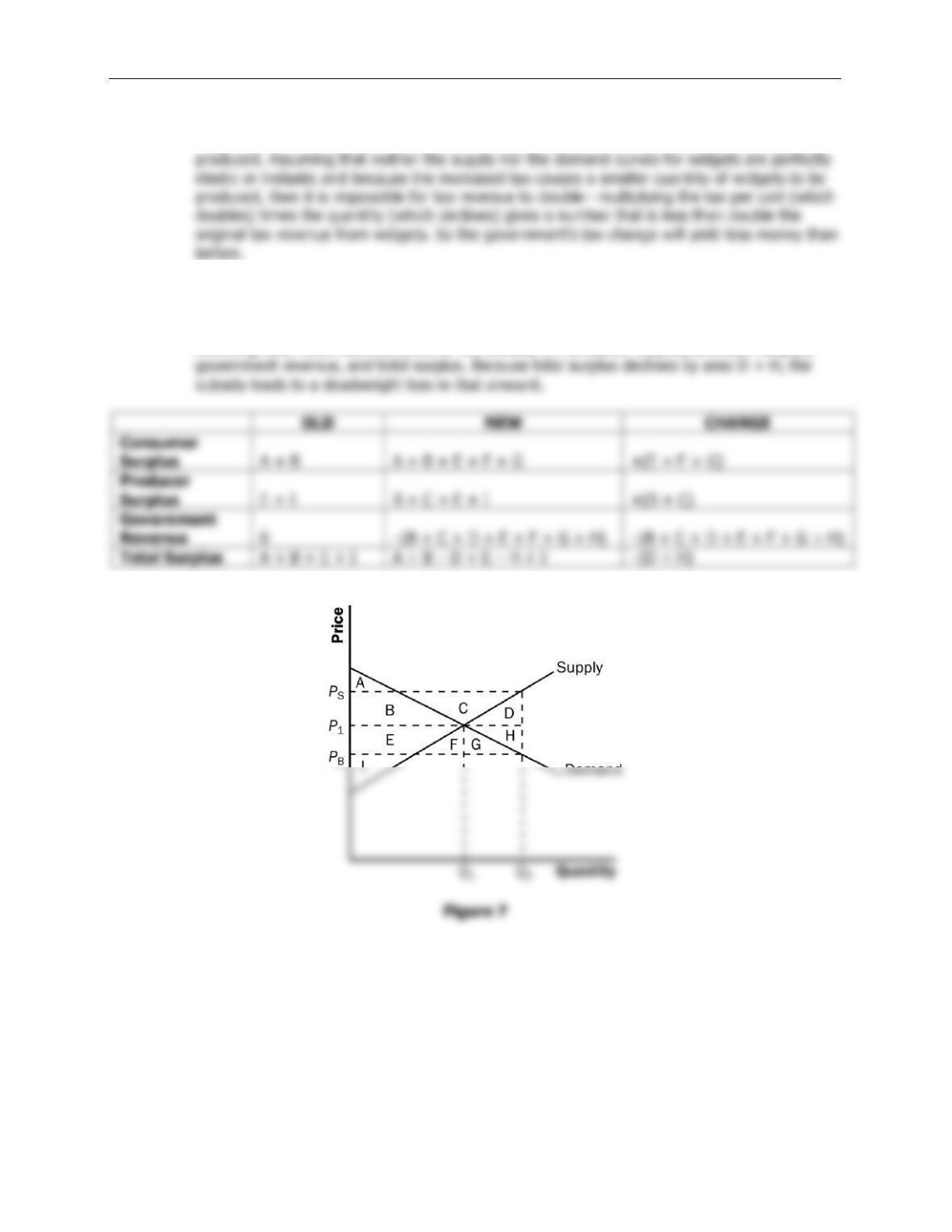
a. Consumer surplus is equal to: A + B + C.
Figure 2
Figure 3
If you spent enough time covering consumer and producer surplus in Chapter 7,
students should have an easy time with this concept.
Chapter 8 /Application: The Costs of Taxation ❖ 147
5. Changes in Welfare
a. Consumer surplus changes by: –(B + C).
6. Definition of deadweight loss: the fall in total surplus that results from a market
distortion, such as a tax.
D. Deadweight Losses and the Gains from Trade
1. Taxes cause deadweight losses because they prevent buyers and sellers from benefiting from
trade.
3. The deadweight loss is equal to areas C and E (the drop in total surplus).
Figure 4
148 ❖ Chapter 8 /Application: The Costs of Taxation
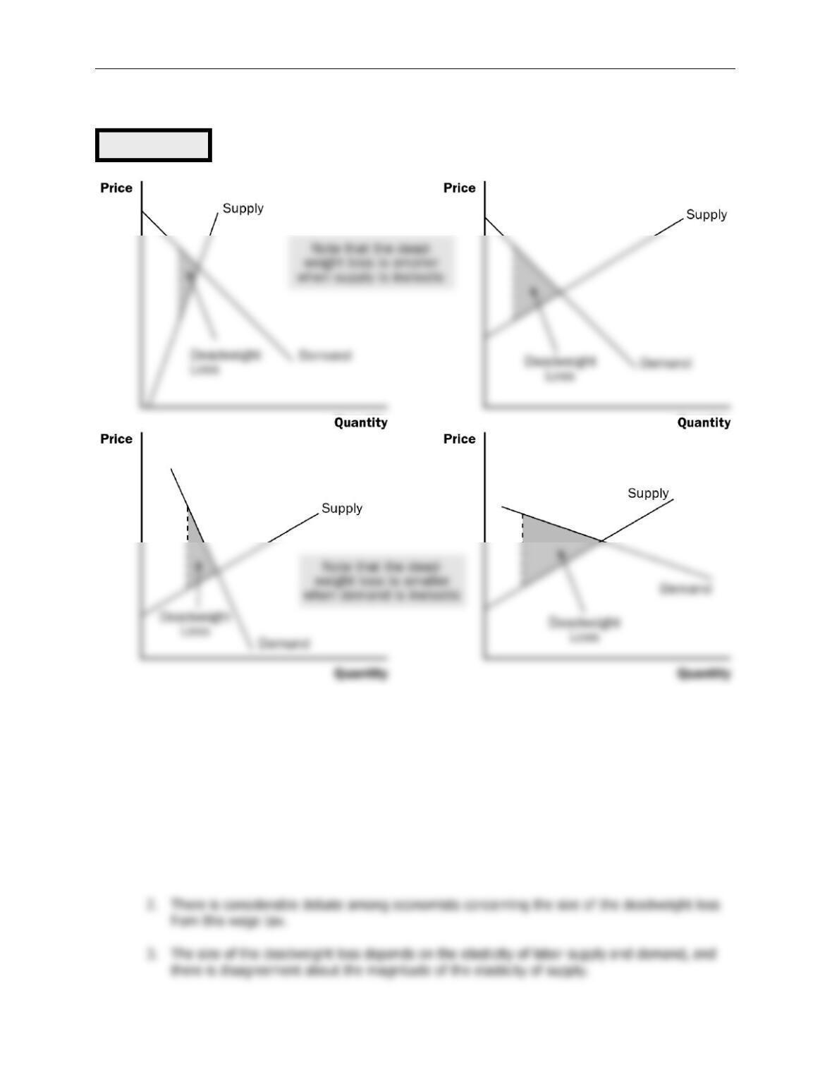
II. The Determinants of the Deadweight Loss
A. The price elasticities of supply and demand will determine the size of the deadweight loss that
occurs from a tax.
1. Given a stable demand curve, the deadweight loss is larger when supply is relatively elastic.
2. Given a stable supply curve, the deadweight loss is larger when demand is relatively elastic.
B.
Case Study: The Deadweight Loss Debate
1. Social Security tax and federal income tax are taxes on labor earnings. A labor tax places a
tax wedge between the wage the firm pays and the wage that workers receive.
Figure 5

Chapter 8 /Application: The Costs of Taxation ❖ 149
a. Economists who argue that labor taxes do not greatly distort market outcomes believe
that labor supply is fairly inelastic.
b. Economists who argue that labor taxes lead to large deadweight losses believe that labor
supply is more elastic.
III. Deadweight Loss and Tax Revenue as Taxes Vary
A. As taxes increase, the deadweight loss from the tax increases.
B. In fact, as taxes increase, the deadweight loss rises more quickly than the size of the tax.
Activity 1—Labor Taxes
Type: In-class discussion
Topics: Deadweight loss, taxation
Materials needed: None
Time: 10 minutes
Class limitations: Works in any size class
Purpose
Most students have not spent a great deal of time considering the effects of taxation on labor
supply. This in-class exercise gives them the opportunity to consider the effects of proposed
tax rates on their own willingness to supply labor.
Instructions
Ask students to assume that they are full-time workers earning $10 per hour, $80 per day,
$400 per week, $20,000 per year.
Points for Discussion
Many students have no idea that current marginal tax rates are greater than 30% for many
taxpayers.
Figure 6
150 ❖ Chapter 8 /Application: The Costs of Taxation
2. If we double the size of a tax, the base and height of the triangle both double so the area of
the triangle (the deadweight loss) rises by a factor of four.
D.
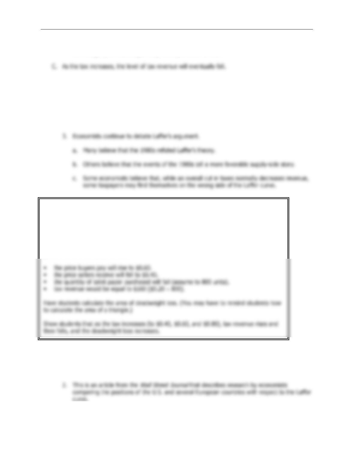
Case Study: The Laffer Curve and Supply-Side Economics
1. The relationship between the size of a tax and the level of tax revenues is called a Laffer
curve.
2. Supply-side economists in the 1980s used the Laffer curve to support their belief that a drop
in tax rates could lead to an increase in tax revenue for the government.
E.
In the News:
New Research on Taxation
1. The latest economic research indicates that some European countries may be on the
declining side of the Laffer curve.
ALTERNATIVE CLASSROOM EXAMPLE:
Draw a graph showing the demand and supply of paper clips. (Draw each curve as a 45–
degree line so that buyers and sellers will share any tax equally.) Mark the equilibrium price
as $0.50 (per box) and the equilibrium quantity as 1,000 boxes. Show students the areas of
producer and consumer surplus.
Impose a $0.20 tax on each box. Assume that sellers are required to “pay” the tax to the
government. Show students that:
Chapter 8 /Application: The Costs of Taxation ❖ 151
Activity 2—Tax Alternatives
Type: In-class assignment
Topics: Taxes and deadweight loss
Materials needed: None
Time: 20 minutes
Class limitations: Works in any size class
Purpose
The market impact of taxes can be a new concept to many students. This exercise helps them
think about the effects of taxes on different goods. Taxes that may be appealing for equity
reasons can be distortionary from a market perspective.
Instructions
Tell the class, “The state has decided to increase funding for public education. They are
considering four alternative taxes to finance these expenditures. All four taxes would raise the
same amount of revenue.” List these options on the board:
1. A sales tax on food.
2. A tax on families with school-age children.
Common Answers and Points for Discussion
A. Taxes change incentives. How might individuals change their behavior because of
each of these taxes?
1. A sales tax on food: At the margin, some consumers will purchase less food.
Overall food purchases will not decrease substantially because the tax will be
spread over a large number of consumers and demand is relatively inelastic.
2. A tax on families with school-age children: No families would put their children up
152 ❖ Chapter 8 /Application: The Costs of Taxation
SOLUTIONS TO TEXT PROBLEMS:
Quick Quizzes
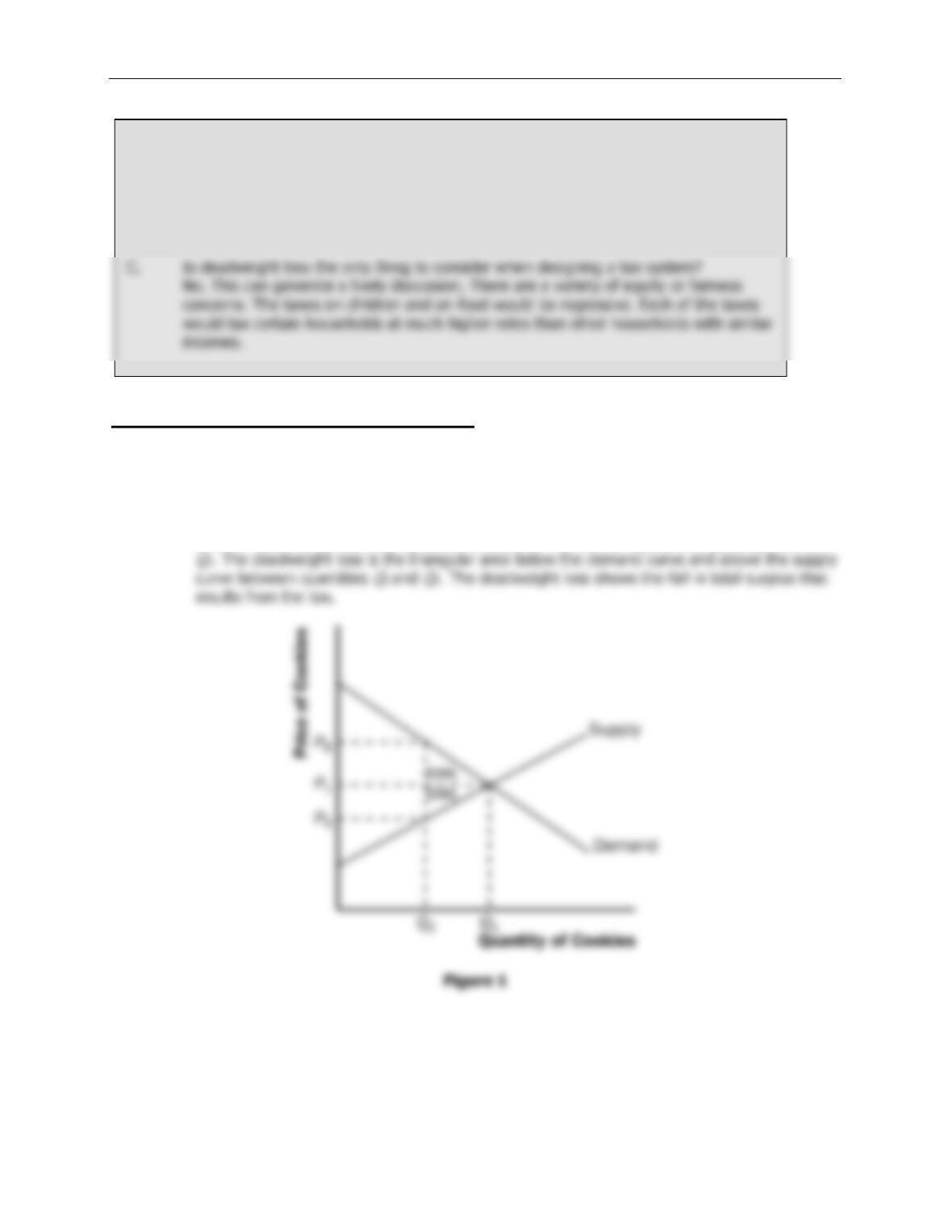
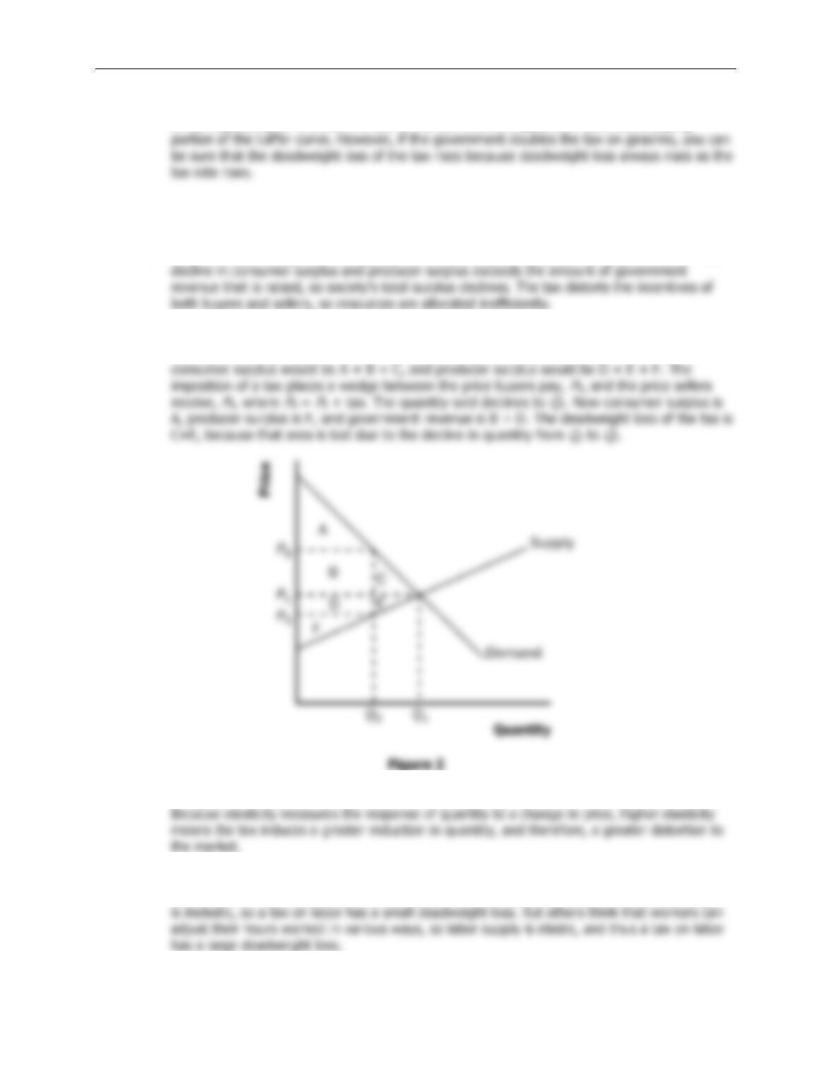
1. Figure 1 shows the supply and demand curves for cookies, with equilibrium quantity
Q
1 and
equilibrium price
P
1. When the government imposes a tax on cookies, the price to buyers
rises to
P
B, the price received by sellers declines to
P
S, and the equilibrium quantity falls to
2. The deadweight loss of a tax is greater the greater is the elasticity of demand. Therefore, a
tax on beer would have a larger deadweight loss than a tax on milk because the demand for
beer is more elastic than the demand for milk.
B. Rank these taxes from smallest deadweight loss to largest deadweight loss.
Lowest deadweight loss—tax on children, very inelastic.
Then—tax on food. Demand is inelastic; supply is elastic.
Third—tax on vacation homes. Demand is elastic; short-run supply is inelastic.
Most deadweight loss—tax on jewelry. Demand is elastic; supply is elastic.
Chapter 8 /Application: The Costs of Taxation ❖ 153
3. If the government doubles the tax on gasoline, the revenue from the gasoline tax could rise
or fall depending on whether the size of the tax is on the upward or downward sloping
Questions for Review
1. When the sale of a good is taxed, both consumer surplus and producer surplus decline. The
2. Figure 2 illustrates the deadweight loss and tax revenue from a tax on the sale of a good.
Without a tax, the equilibrium quantity would be
Q
1, the equilibrium price would be
P
1,
3. The greater the elasticities of demand and supply, the greater the deadweight loss of a tax.
4. Experts disagree about whether labor taxes have small or large deadweight losses because
they have different views about the elasticity of labor supply. Some believe that labor supply
154 ❖ Chapter 8 /Application: The Costs of Taxation
5. The deadweight loss of a tax rises more than proportionally as the tax rises. Tax revenue,
however, may increase initially as a tax rises, but as the tax rises further, revenue eventually
declines.
Problems and Applications
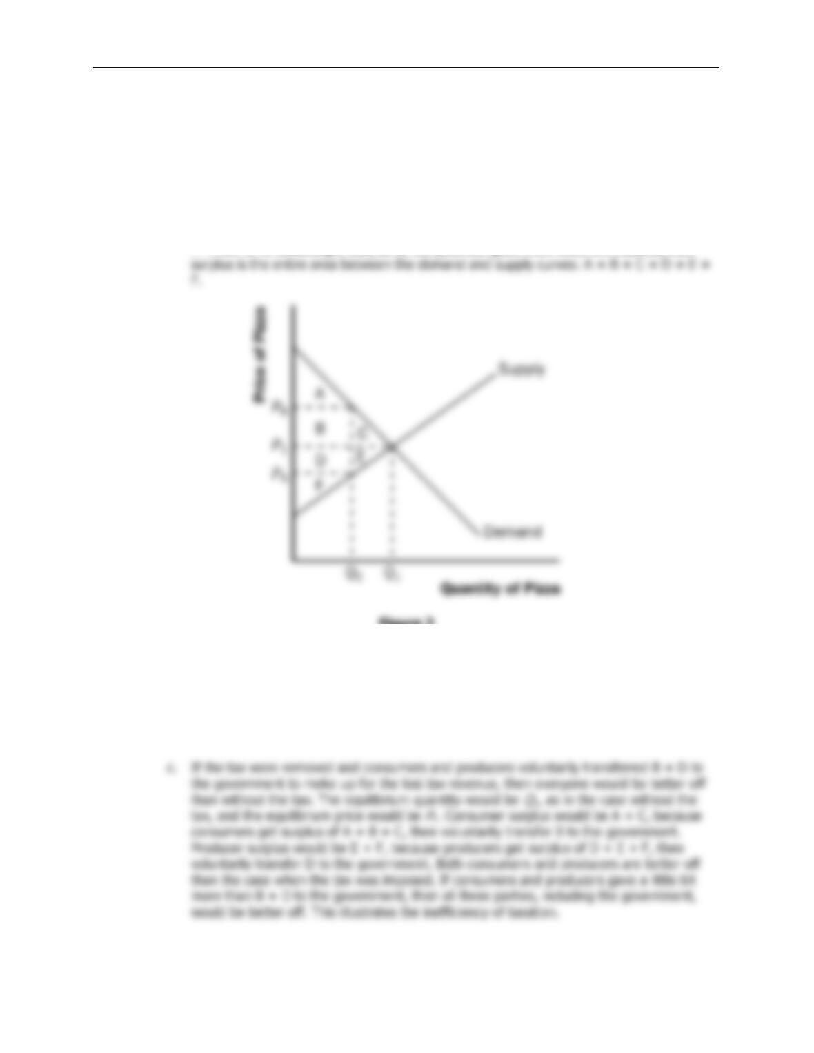
1. a. Figure 3 illustrates the market for pizza. The equilibrium price is
P
1, the equilibrium
quantity is
Q
1, consumer surplus is area A + B + C, and producer surplus is area D + E +
F. There is no deadweight loss, as all the potential gains from trade are realized; total
Figure 3
b. With a $1 tax on each pizza sold, the price paid by buyers,
P
B, is now higher than the
price received by sellers,
P
S, where
P
B =
P
S + $1. The quantity declines to
Q
2, consumer
surplus is area A, producer surplus is area F, government revenue is area B + D, and
deadweight loss is area C + E. Consumer surplus declines by B + C, producer surplus
declines by D + E, government revenue increases by B + D, and deadweight loss
increases by C + E.
Chapter 8 /Application: The Costs of Taxation ❖ 155
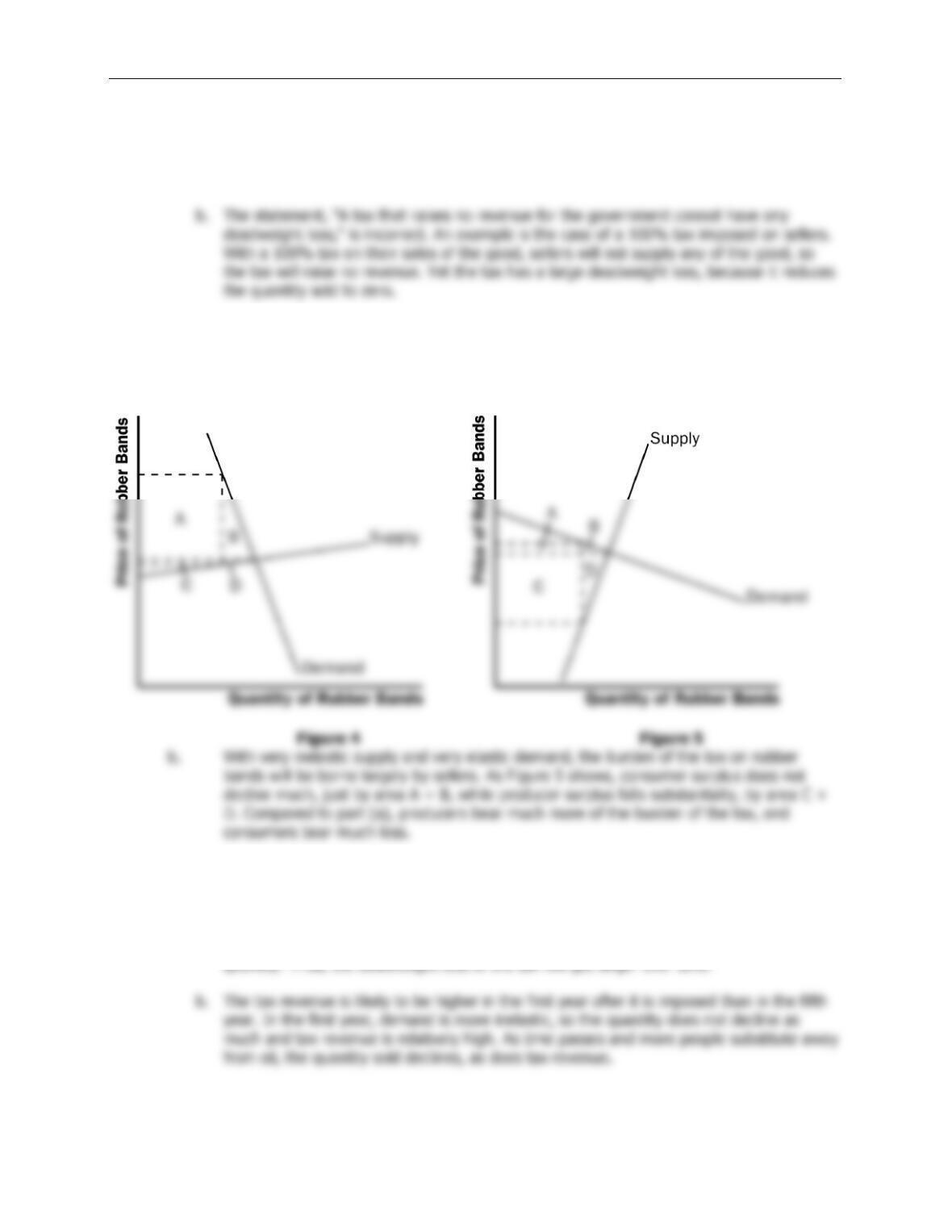
2. a. The statement, “A tax that has no deadweight loss cannot raise any revenue for the
government,” is incorrect. An example is the case of a tax when either supply or demand
is perfectly inelastic. The tax has neither an effect on quantity nor any deadweight loss,
but it does raise revenue.
3. a. With very elastic supply and very inelastic demand, the burden of the tax on rubber
bands will be borne largely by buyers. As Figure 4 shows, consumer surplus declines
considerably, by area A + B, but producer surplus does not fall much at all, just by area
C + D.
4. a. The deadweight loss from a tax on heating oil is likely to be greater in the fifth year after
it is imposed rather than the first year. In the first year, the elasticity of demand is fairly
low, as people who own oil heaters are not likely to get rid of them right away. But over
time they may switch to other energy sources and people buying new heaters for their
homes will more likely choose gas or electric, so the tax will have a greater impact on
156 ❖ Chapter 8 /Application: The Costs of Taxation
5. Because the demand for food is inelastic, a tax on food is a good way to raise revenue
because it does not lead to much of a deadweight loss; thus taxing food is less inefficient
6. a. This tax has such a high rate that it is not likely to raise much revenue. Because of the
7. a. Figure 6 illustrates the market for socks and the effects of the tax. Without a tax, the
equilibrium quantity would be
Q
1, the equilibrium price would be
P
1, total spending by
consumers equals total revenue for producers, which is
P
1 x
Q
1, which equals area B + C
+ D + E + F, and government revenue is zero. The imposition of a tax places a wedge
between the price buyers pay,
P
B, and the price sellers receive,
P
S, where
P
B =
P
S + tax.
The quantity sold declines to
Q
2. Now total spending by consumers is
P
B x
Q
2, which
equals area A + B + C + D, total revenue for producers is
P
S x
Q
2, which is area C + D,
and government tax revenue is
Q
2 x tax, which is area A + B.
c. The price paid by consumers rises, unless demand is perfectly elastic or supply is
perfectly inelastic. Whether total spending by consumers rises or falls depends on the
price elasticity of demand. If demand is elastic, the percentage decline in quantity
Chapter 8 /Application: The Costs of Taxation ❖ 157
8. Because the tax on gadgets was eliminated, all tax revenue must come from the tax on
widgets. The tax revenue from the tax on widgets equals the tax per unit times the quantity
9. Figure 7 illustrates the effects of the $2 subsidy on a good. Without the subsidy, the
equilibrium price is
P
1 and the equilibrium quantity is
Q
1. With the subsidy, buyers pay price
P
B, producers receive price
P
S (where
P
S =
P
B + $2), and the quantity sold is
Q
2. The
following table illustrates the effect of the subsidy on consumer surplus, producer surplus,
158 ❖ Chapter 8 /Application: The Costs of Taxation
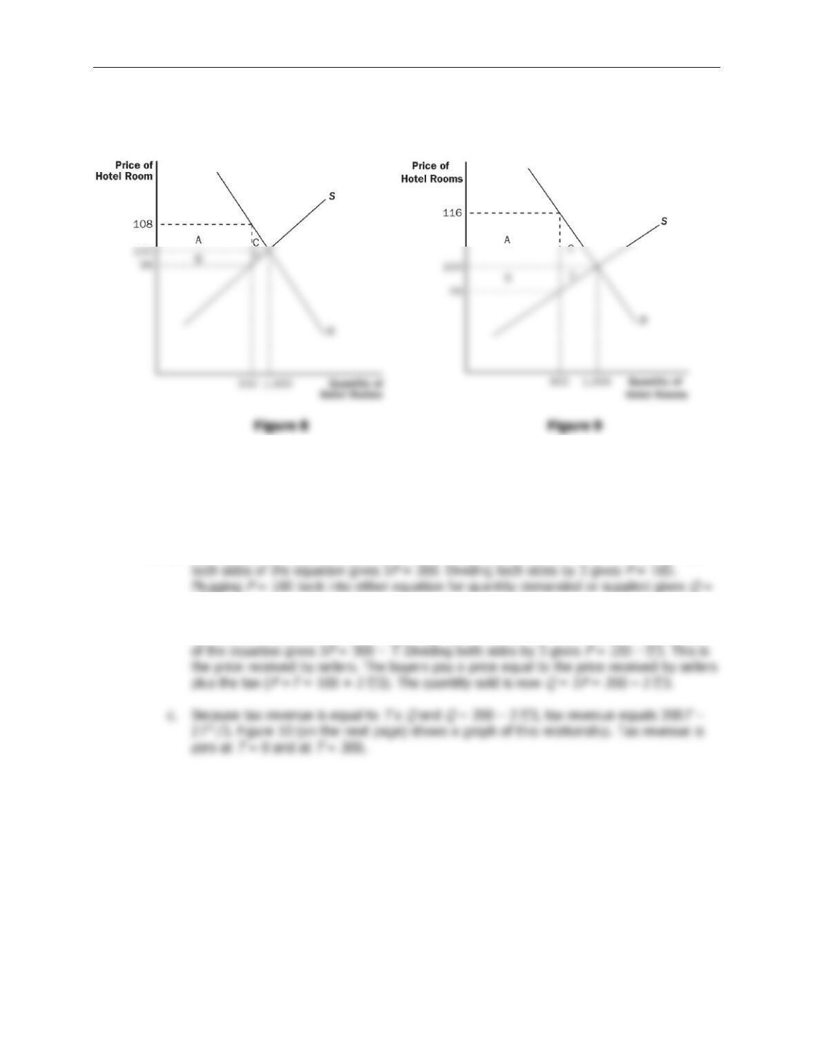
10. a. Figure 8 shows the effect of a $10 tax on hotel rooms. The tax revenue is represented by
areas A + B, which are equal to ($10)(900) = $9,000. The deadweight loss from the tax
is represented by areas C + D, which are equal to (0.5)($10)(100) = $500.
b. Figure 9 shows the effect of a $20 tax on hotel rooms. The tax revenue is represented by
areas A + B, which are equal to ($20)(800) = $16,000. The deadweight loss from the tax
is represented by areas C + D, which are equal to (0.5)($20)(200) = $2,000.
When the tax is doubled, the tax revenue rises by less than double, while the deadweight
loss rises by more than double.
11. a. Setting quantity supplied equal to quantity demanded gives 2
P
= 300 –
P
. Adding
P
to
200.
b. Now P is the price received by sellers and
P
+
T
is the price paid by buyers. Equating
quantity demanded to quantity supplied gives
2P
= 300 − (
P
+
T
). Adding
P
to both sides
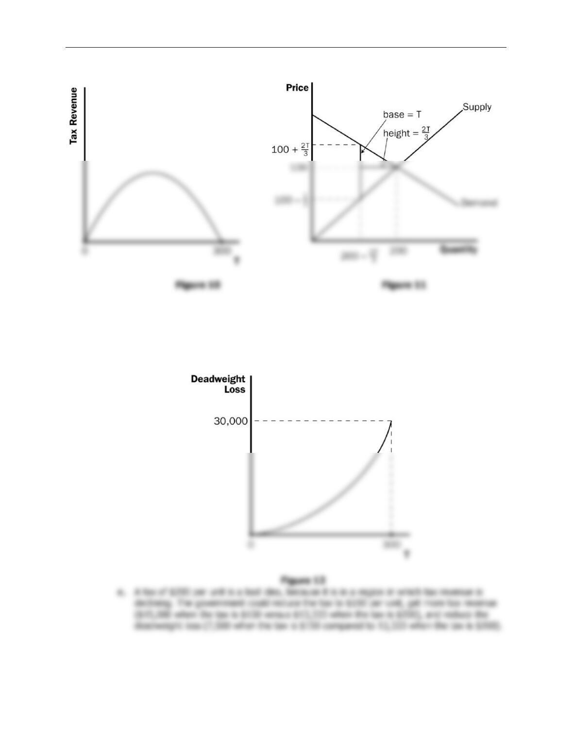
Chapter 8 /Application: The Costs of Taxation ❖ 159
d. As Figure 11 shows, the area of the triangle (laid on its side) that represents the
deadweight loss is 1/2 × base × height, where the base is the change in the price, which
is the size of the tax (
T
) and the height is the amount of the decline in quantity (2
T
/3).
So the deadweight loss equals 1/2 ×
T
× 2
T
/3 =
T
2/3. This rises exponentially from 0
(when
T
= 0) to 30,000 when
T
= 300, as shown in Figure 12.