Chapter 8 A concrete cutoff wall will be built as shown

Chapter 8

Groundwater—Multidimensional Flow and

Applications

SOLUTIONS TO QUESTIONS AND PRACTICE PROBLEMS

Section 8.2 Flow Net Solutions for Two-Dimensional Flow

8.1 One of the factors in Equation 8.27 is NF, yet when drawing a flow net we assume a

value for this parameter. How can this formula produce correct results when one of the

factors is assumed? (i.e., would assuming a higher NF produce a higher computed value

of Q?)

Solution

Equation 8.26 is expressed in terms of the ratio NF/ND, and it is this ratio that is a constant

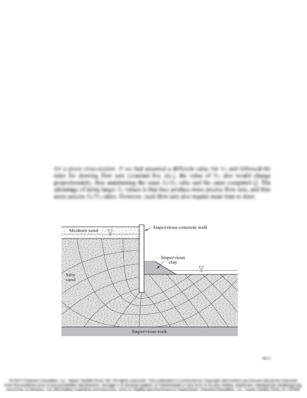
8.2 The flow net in Figure 8.38 is incorrect. Explain why.

Figure 8.38 Trial flow net for Problem 8.2. Note: This flow net is not drawn correctly

and should not be used as an example!

8-2 Groundwater—Multidimensional Flow and Applications Chap. 8

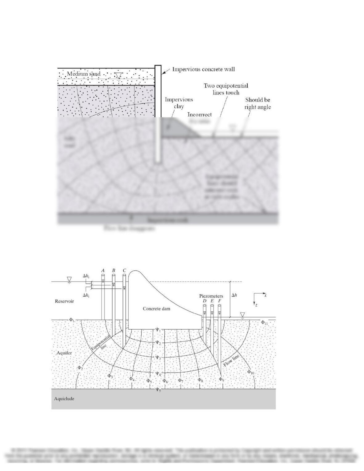
Solution

This flow net has many problems. The major ones are shown in the following figure.

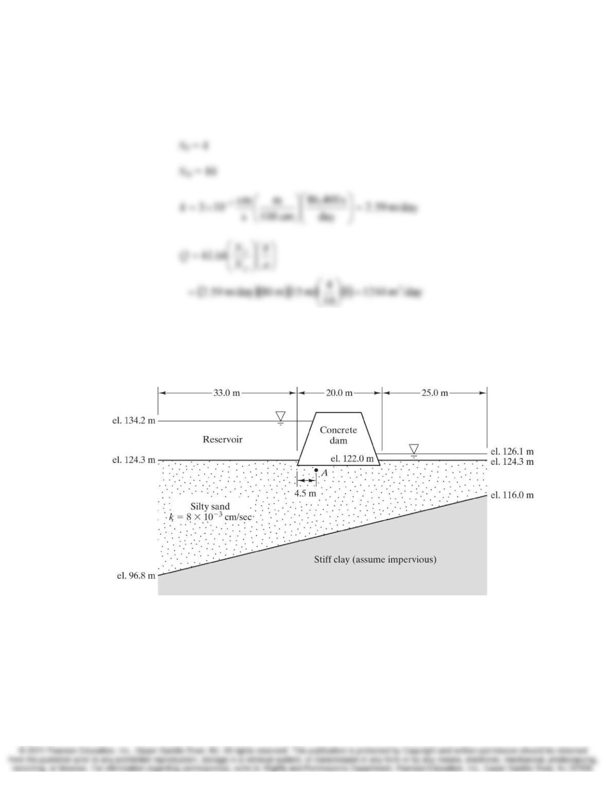
8.3 Compute the total flow rate under the dam shown in Figure 8.2 under the following

conditions: Δh = 15 m, the soil beneath the dam has a hydraulic conductivity of 3×10-3

cm/s, and the length of the dam into the page is 80 m.

Figure 8.2 A sample flow net of seepage beneath a concrete dam

Chap. 8 Groundwater—Multidimensional Flow and Applications 8-3

Solution

From Figure 8.2:

b/a=1

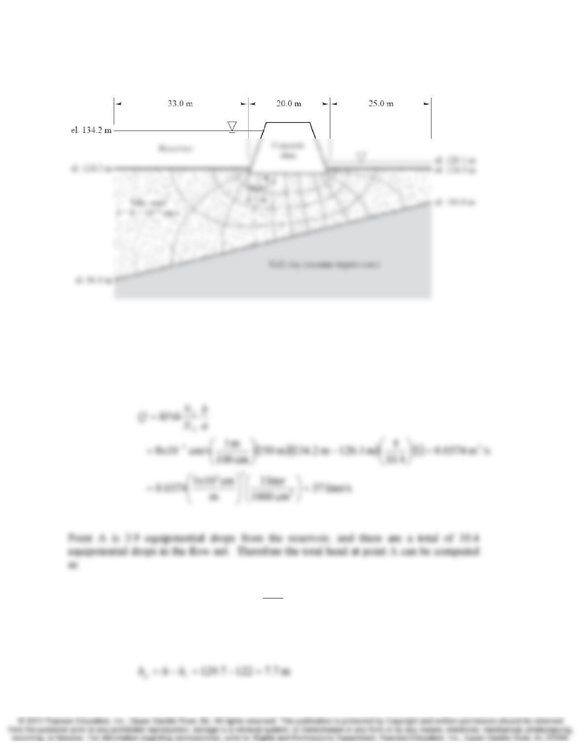
8.4 Redraw the cross-section in Figure 8.39 to a scale of 1:500 (1 cm = 5 m), then draw a

flow net that describes the seepage below this 150 m long concrete dam. Finally,

compute the flow rate through this soil, expressed in liters per second, and the pore water

pressure at Point A, which is at elevation 122.0 m.

Figure 8.39 Cross-section of dam for Problems 8.4 and 8.5. el. = elevation

8-4 Groundwater—Multidimensional Flow and Applications Chap. 8

Solution

Based on flow net:

NF=4

ND=10.4 note: the last equipotential drop on the right side is

approximated 0.4×a full drop

()

m 129.7

4.10

6.3

1.1262.1342.134 =

⎟

⎠

⎞

⎜

⎝

⎛

−−=h

Scaling from the drawing, the elevation at A is 122 m. Therefore the pressure head and

pore water pressure at A are computed as

Chap. 8 Groundwater—Multidimensional Flow and Applications 8-5

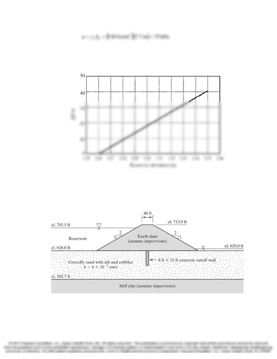
8.5 Using the flow net from Problem 8.4, develop a plot of seepage flow rate vs. the water

elevation in the reservoir. Consider reservoir elevations between 126.1 m and 135.0 m.

Solution

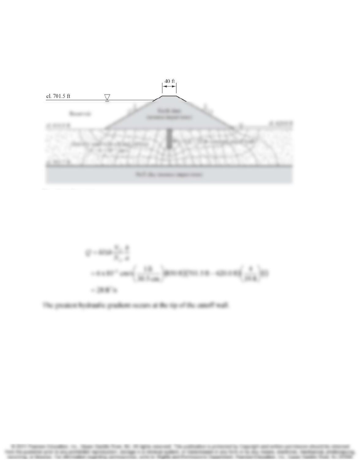
8.6 The earth dam shown in Figure 8.40 is to be built on a gravelly sand with silt and cobbles.

This dam will extend a distance of 850 ft perpendicular to the cross-section. To reduce

the flow rate through these soils, a concrete cutoff wall will be built as shown. Redraw

this cross-section to a scale of 1 in = 100 ft, draw a flow net, and compute Q. Then,

identify the area in the flow net that has the greatest hydraulic gradient.

Figure 8.40 Cross-section for Problem 8.6. el. = elevation

8-6 Groundwater—Multidimensional Flow and Applications Chap. 8

Solution

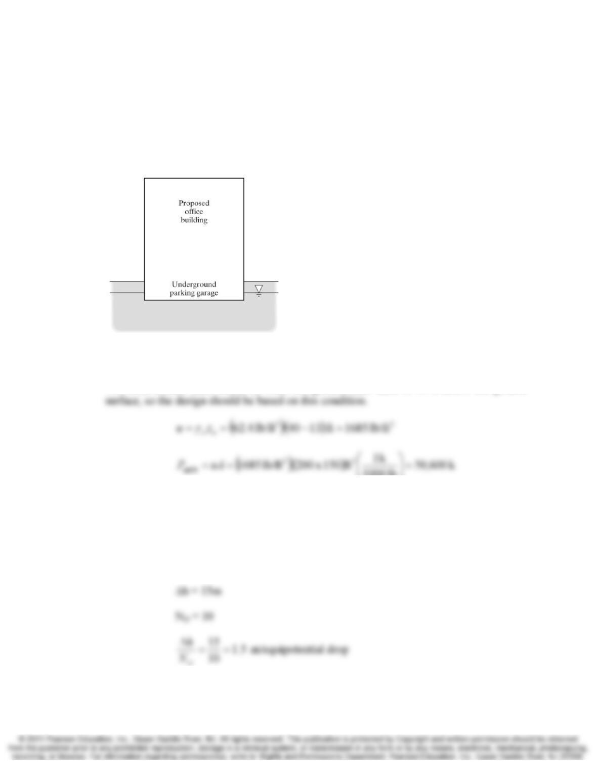
Completed flow net

Based on flow net:

NF=4

ND=19.8 note: the last equipotential drop on the right side is

approximated 0.8×a full drop

Chap. 8 Groundwater—Multidimensional Flow and Applications 8-7

8.7 A proposed twenty-story office building with three levels of underground parking will be

supported on a concrete mat foundation, as shown in Figure 8.41. The bottom of this mat

will be 40 ft below the street, and its plan dimensions will be 200 ft × 150 ft. The

groundwater table is currently at a depth of 25 ft below the ground surface, but could rise

to only 13 ft below the ground surface during the life of the building. Compute the total

hydrostatic uplift force to be used in the design.

Figure 8.41 Proposed underground parking area for Problem 8.7.

Solution

The most critical case would be when the groundwater table is 13 ft below the ground

lb 1000

⎠

⎝

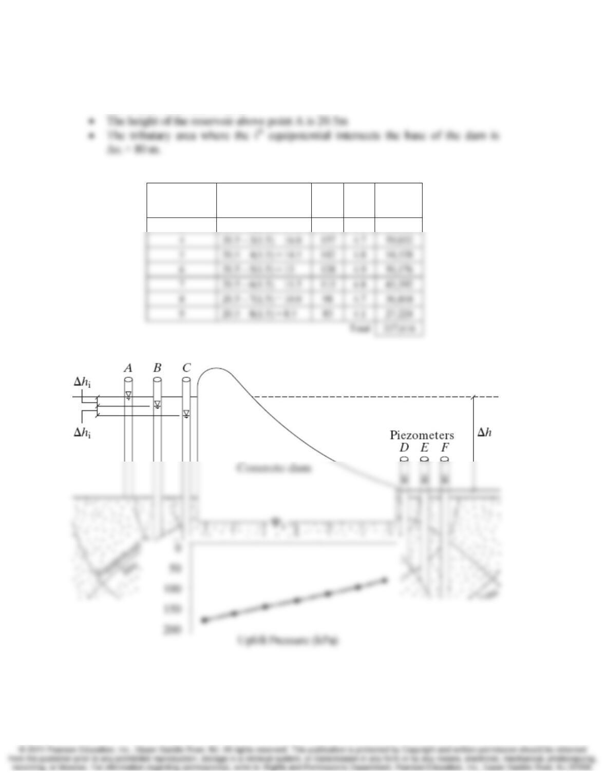
8.8 Compute the uplift forces acting on the dam in Figure 8.2 using the data in Problem 8.3.

Draw a diagram of the uplift pressure acting on the dam and compute the total uplift force.

Solution

Using the information from 8.3:

8-8 Groundwater—Multidimensional Flow and Applications Chap. 8

Taking datum to be the lower left corner of the dam, point A shown below, and setting

Δh = 15m:

• The width of the dam is 32 m

The pressures and forces along the base of the dam are then computed as:

Equipotential

drop Δh (m) u

(kPa)

Δxi

(m)

Upliift

Force

(kN)

3 20.5 – 2(1.5) = 17.5 172 4.1 56,416

Chap. 8 Groundwater—Multidimensional Flow and Applications 8-9

8.9 The sheet pile in Example 8.5 was located near the upstream end of the spillway. Would

the total hydrostatic uplift force acting on the structure change if the sheet pile was

located near the downstream end? Explain. Which position would be best? Why?

Solution

Since the groundwater must pass through a narrow opening beneath the sheet pile, there

is extra head loss in this vicinity. Therefore, the uplift pressure immediately downstream

Section 8.3 Numerical Modeling of Two-Dimensional Flow

For problems 8.10 and 8.11, see Appendix D for guidance on finite difference solutions

to flow problems.

8.10 Create a finite difference model for the sheet pile system shown in Figure 8.4 using a

commercial spreadsheet program. Plot the equipotential lines using you program and

sketch in the flow lines. Compare your solution to that shown in Figure 8.4. If the

hydraulic conductivity of the soil in the aquifer is 2×10-4 cm/s, what is the total flow rate

per meter of wall length into the page?

Solution

An example finite difference solution is provided in the files

8.11 Create a finite difference model for the spillway with cutoff wall shown in Figure 8.9

using a commercial spreadsheet program. Plot the equipotential lines within the aquifer

as well as the uplift forces on the base of the spillway. Compare your results to those

shown in Example 8.5.

Solution

An example finite difference solution is provided in the files

8-10 Groundwater—Multidimensional Flow and Applications Chap. 8

Section 8.4 Two and Three Dimensional Flow to Wells

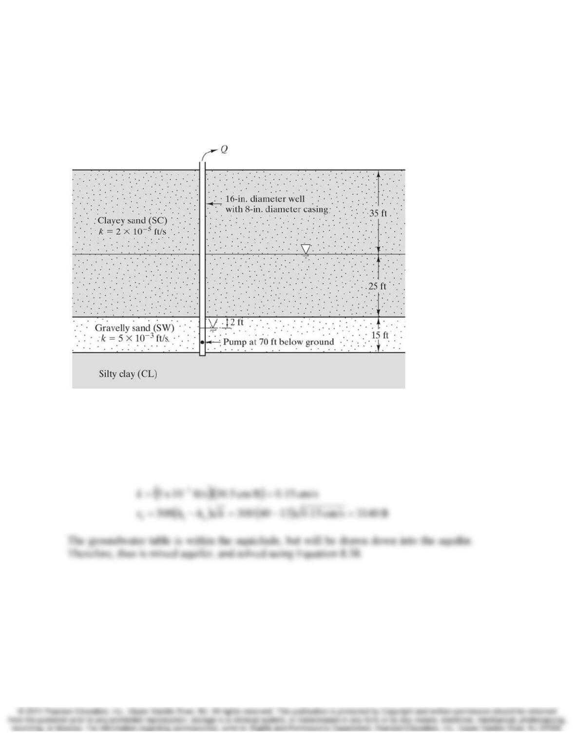
8.12 The proposed well shown in Figure 8.42 will be used to supply a municipal water system.

Compute its pumping capacity with the groundwater level as shown, and express your

answer in gallons per minute.

Figure 8.42 Proposed well for Problems 8.12 and 8.13.

Solution

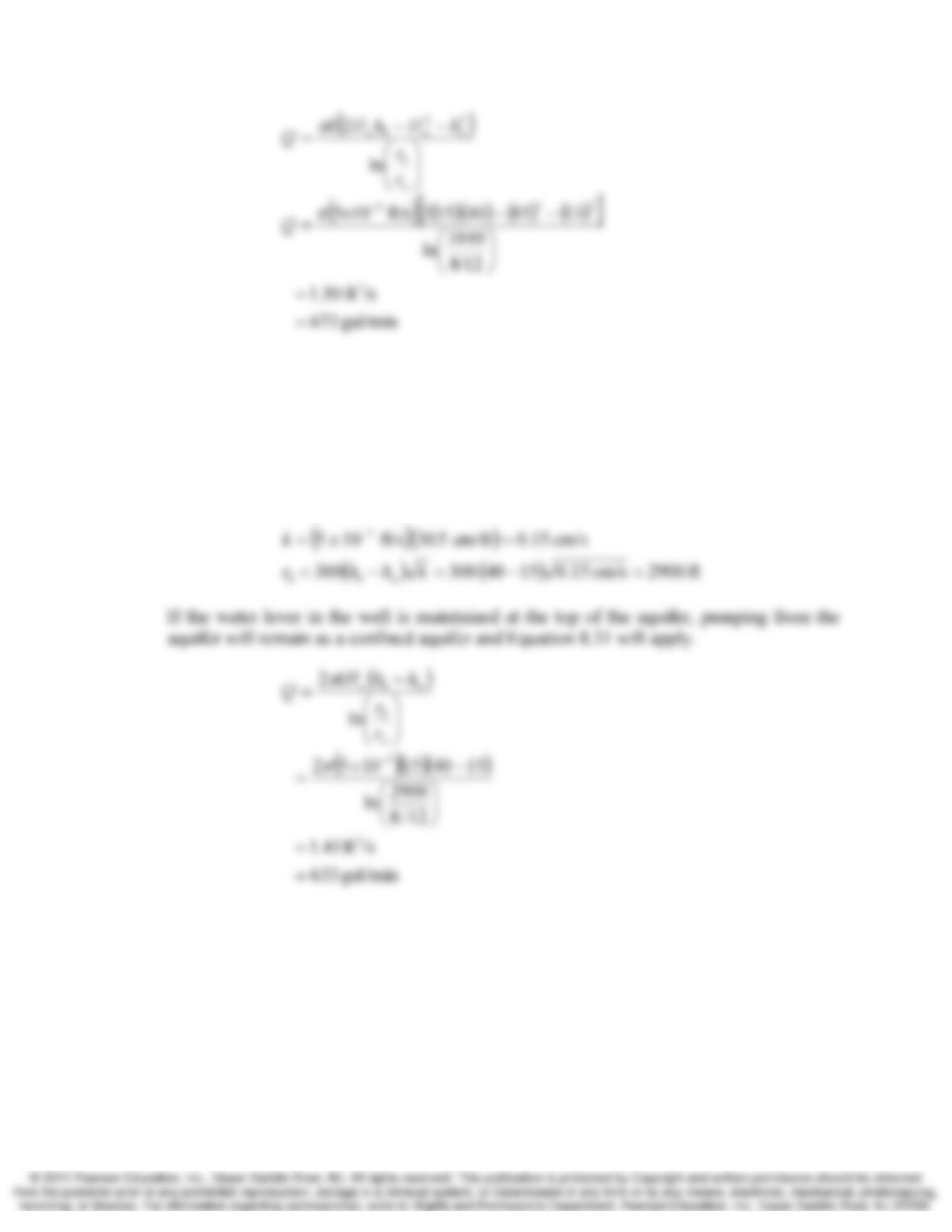
We have no information about a recharge source so we must estimate r0 using Equation

8.34

Chap. 8 Groundwater—Multidimensional Flow and Applications 8-11

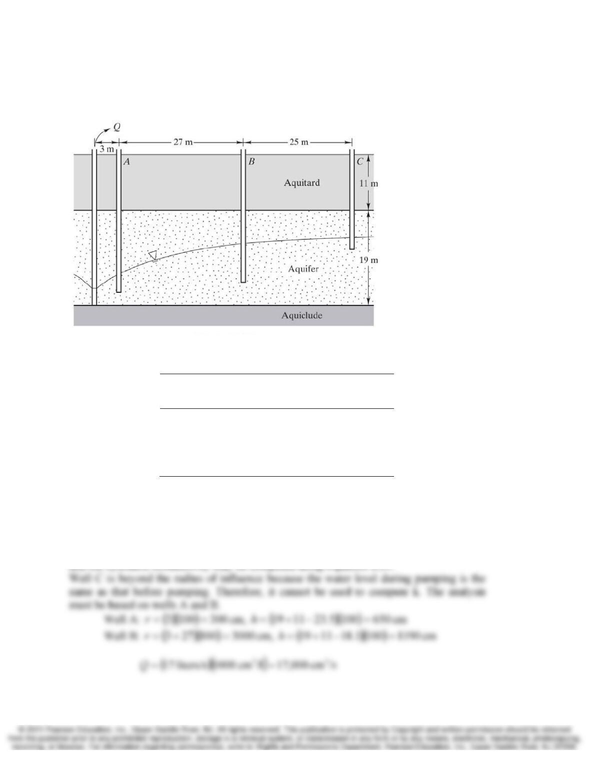
8.13 Using the well shown in Figure 8.42, if the drawdown is limited such that the level of

water in the well is maintained at the top of the gravelly sand layer, what pumping rate is

possible? Express your answer in gallons per minute.

Solution

We have no information about a recharge source so we must estimate r0 using Equation

8.34

8-12 Groundwater—Multidimensional Flow and Applications Chap. 8

8.14 After reaching steady-state conditions, the test well shown in Figure 8.43 is producing a

flow rate of 17 l/s. The aquifer is an alluvial soil with interbedded medium-to-coarse

sand and silty sand.

Figure 8.43 Cross-section for Problems 8.14 and 8.15

The water depths in the observation wells are as follows:

Well Water Depth From Ground Surface (m)

Before Pumping During Pumping

Pumping 16.9 26.0

Observation A 16.9 23.5

Observation B 16.9 18.1

Observation C 16.9 16.9

Using the best available data, compute the hydraulic conductivity of the soil in the

aquifer. Is the computed k value reasonable? Explain why or why not.

Solution

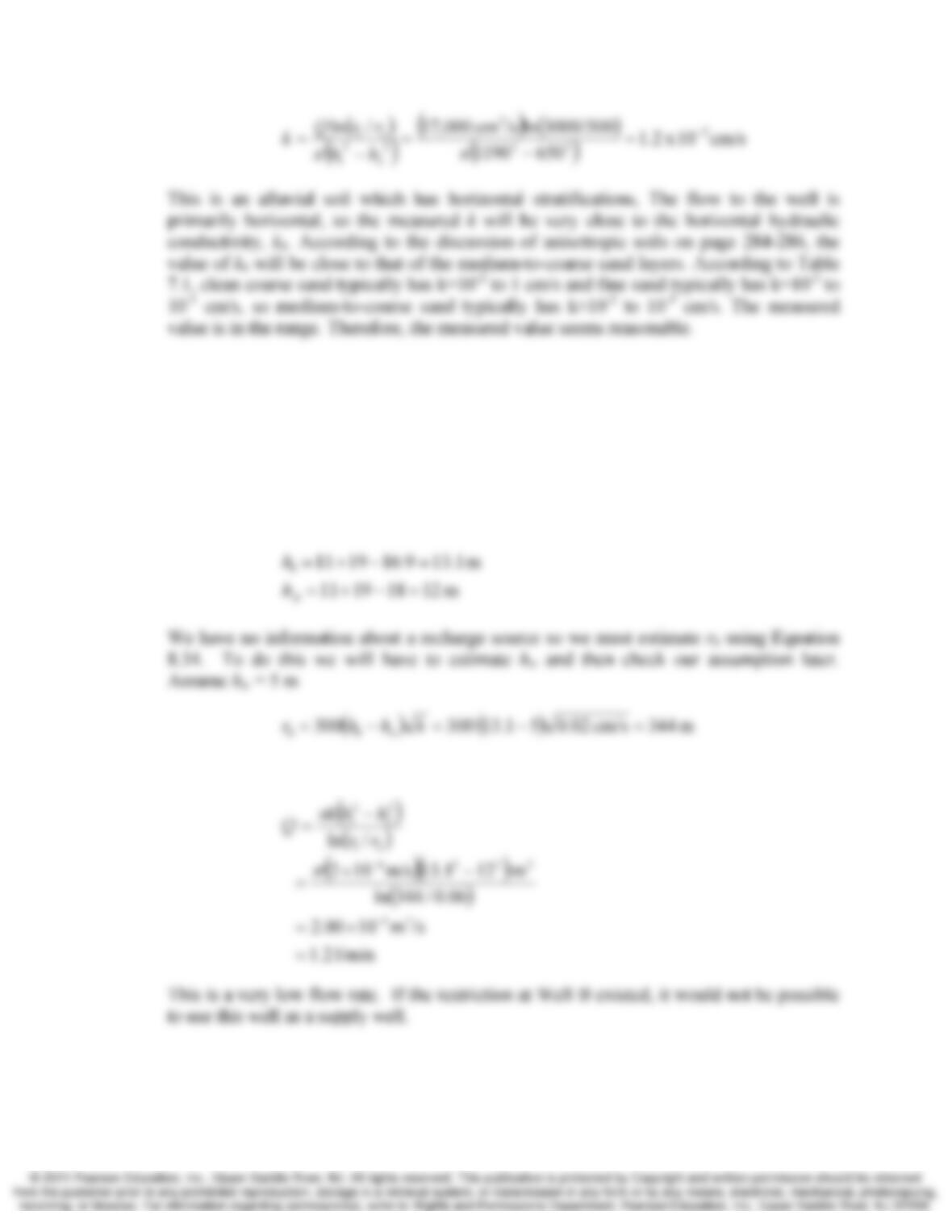
The groundwater table is completely within the aquifer, so this is an unconfined aquifer

Chap. 8 Groundwater—Multidimensional Flow and Applications 8-13

8.15 For the well shown in Figure 8.43 assume the original depth from the ground surface to

the phreatic surface is 16.9 m and the hydraulic conductivity of the soil in the aquifer is

10-2 cm/s. What is the maximum pumping rate, Q, such that the distance from the ground

surface to the phreatic surface at observation well B is no greater than 18 m? Assume

rw = 0.06 m

Solution

Calculate the distance from the top of the Aquiclude:

Since this is an unconfined aquifer Equation 8.35 will apply.