PROBLEM 7.23 (Cont.)
COMMENTS: (1) In Problem 7.15, we see that, for air cooling and Llens = 400 mm, Tsi = 126 C,
P = 14.3 W. Use of liquid cooling increases the electrical power output to 23.4 W, or 64 percent.
In Problem 7.15 we see the maximum power output to be about 15 W. With liquid cooling and
the heat sink, maximum power output increases to about 420 W, or 2800%. (2) The electric
power is highly sensitive to the size of the concentrator. Initially, the power output increases as
the concentrated irradiation increases, but as the silicon temperature increases the efficiency
PROBLEM 7.24
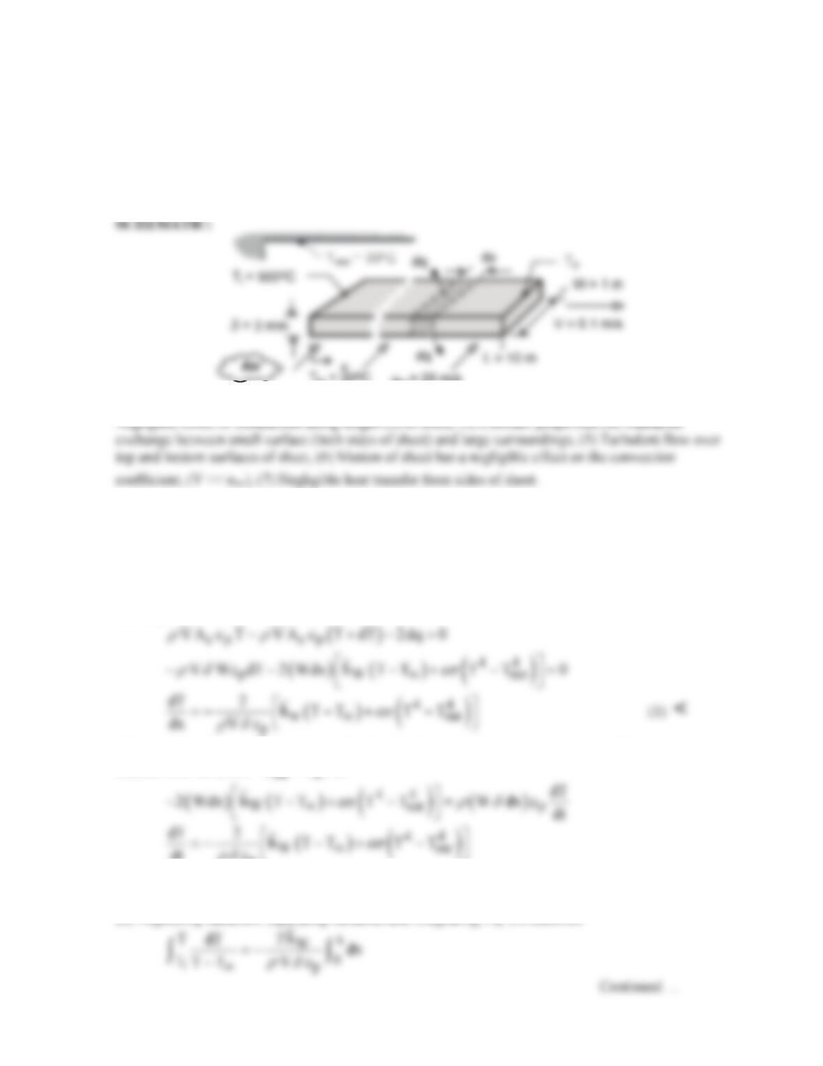
KNOWN: Velocity, initial temperature, properties and dimensions of steel strip on a production line.
Velocity and temperature of air in cross flow over top and bottom surfaces of strip. Temperature of
surroundings.
FIND: (a) Differential equation governing temperature distribution along the strip, (b) Exact solution
for negligible radiation and corresponding value of outlet temperature for prescribed conditions, (c)
Effect of radiation on outlet temperature, and parametric effect of sheet velocity on temperature
distribution.
o
o
u = 20 m/s
o
o
ASSUMPTIONS: (1) Negligible variation of sheet temperature across its width and thickness, (2)
PROPERTIES: Prescribed. Steel:
3
p
7850 kg / m c 620 J / kg K, 0.70.
,
ε
Air: k = 0.044
W/mK,
52
4.5 10 m / s,
Pr = 0.68.
ANALYSIS: (a) Applying conservation of energy to a stationary differential control surface, through
which the sheet passes, conditions are steady and
in out
E E 0.
Hence, with inflow due to advection
and outflow due to advection, convection and radiation
Alternatively, if the control surface is fixed to the sheet, conditions are transient and the energy
balance is of the form,
E E,
or
p
dt c
d
Dividing the left– and right-hand sides of the equation by dx/dt and V = dx/dt, respectively, Eq. (1) is
obtained.
(b) Neglecting radiation, separating variables and integrating, Eq. (1) becomes
PROBLEM 7.24 (Cont.)
With
52 5
W
Re u W / 20 m / s 1m / 4 10 m / s 5 10 ,
the correlation for turbulent flow over a
flat plate yields
Hence, applying Eq. (2) at x = L = 10m,
7850 kg / m 0.1m / s 0.003m 620 J / kg K
(c) Using the DER function of IHT, Eq. (1) may be numerically integrated from x = 0 to x = L = 10m
to obtain
Contrasting this result with that of Part (b), it is clear that radiation makes a discernable contribution
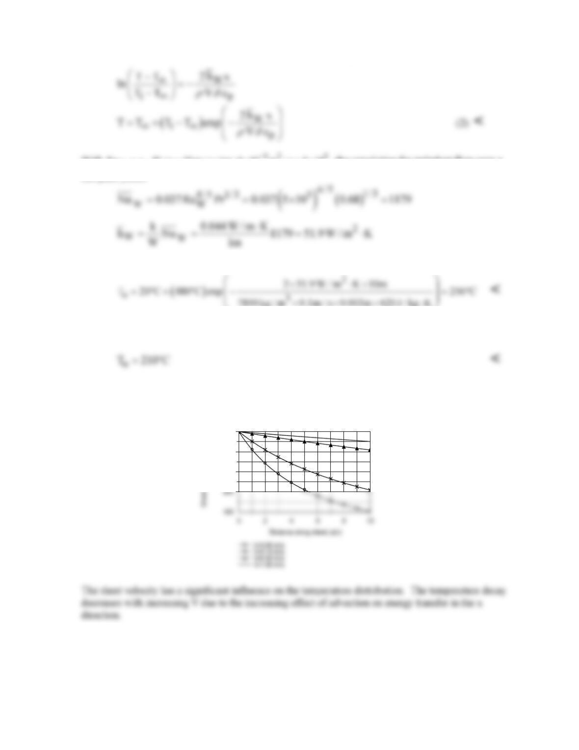
to cooling of the sheet. IHT was also used to determine the effect of the sheet velocity on the
temperature distribution.
COMMENTS: (1) A critical parameter in the production process is the coiling temperature, that is,
the temperature at which the wire may be safely coiled for subsequent storage or shipment. The
larger the production rate (V), the longer the cooling distance needed to achieve a desired coiling
temperature. (2) Cooling may be enhanced by increasing the cross stream velocity u.
300
400
500
PROBLEM 7.25
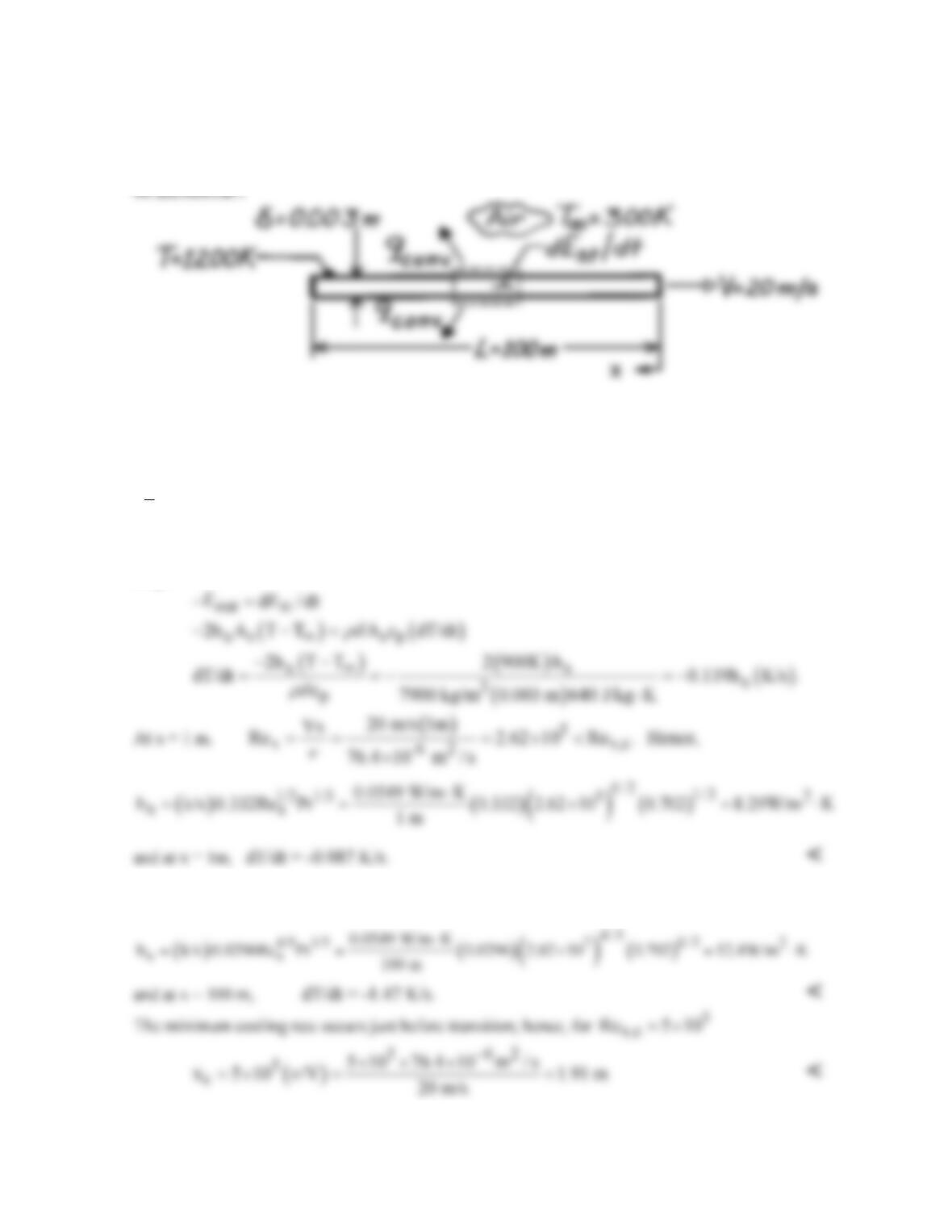
KNOWN: Length, thickness, speed and temperature of steel strip.
FIND: Rate of change of strip temperature 1 m from leading edge and at trailing edge. Location of
minimum cooling rate.
ASSUMPTIONS: (1) Constant properties, (2) Negligible radiation, (3) Negligible longitudinal
conduction in strip, (4) Critical Reynolds number is 5 105.
PROPERTIES: Steel (given): = 7900 kg/m3, cp = 640 J/kgK. Table A-4, Air
T 750K, 1 atm :
= 76.4 10-6 m2/s, k = 0.0549 W/mK, Pr = 0.702.
ANALYSIS: Performing an energy balance for a control mass of unit surface area As riding with the
strip,
At the trailing edge,
7
x x,c
Re 2.62 10 Re . >
Hence
COMMENTS: The cooling rates are very low and would remain low even if radiation were
considered. For this reason, hot strip metals are quenched by water and not by air.
PROBLEM 7.26
KNOWN: Dimensions of flat plate in parallel flow. Plate and fluid temperatures, fluid velocities.
FIND: Average heat transfer coefficient, convection heat transfer rate, drag force for (a) water
flowing at a velocity of 0.5 m/s, (b) nanofluid of Example 2.2 at a velocity of 0.5 m/s, (c) water at a
velocity of 2.5 /m/s, (d) nanofluid at a velocity of 2.5 m/s.
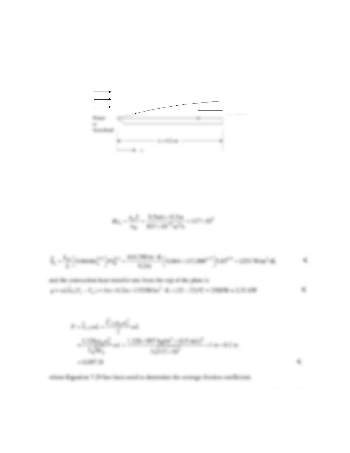
SCHEMATIC:
ASSUMPTIONS: (1) Steady-state conditions, (2) Constant properties, Rex,c = 5 105.
PROPERTIES: Table A.4, water (300 K):
bf = 997 kg/m3,
bf = 857 10-9 m2/s, kbf = 0.613 W/mK,
Prbf = 5.83. Example 2.2, nanofluid (300 K):
nf = 1146 kg/m3,
µ
nf = 962 10-6 m2/s,
nf =
µ
nf/
nf = 839
10-9 m2/s, knf = 0.705 W/mK,
α
nf = 171 10-9 m2/s Prnf =
nf/
α
nf = 4.91.
ANALYSIS: (a) For water flowing over the plate at um = 0.5 m/s,
Since ReL < Rex,c the flow is laminar and Eq. 7.30 yields
The drag force on the plate is
Continued…
T
= 22°C
u
= 0.5 m/s or 2.5 m/s
T
= 32°C
PROBLEM 7.26 (Cont.)
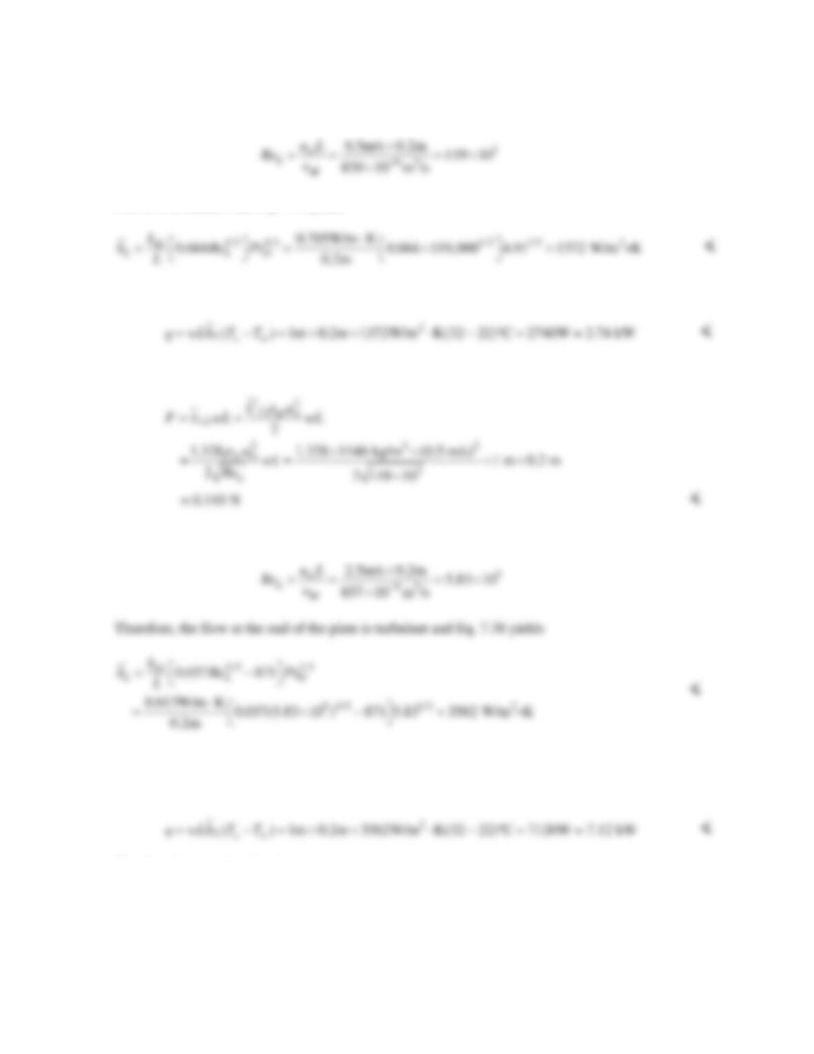
(b) For the nanofluid flowing over the plate at um = 0.5 m/s,
The flow is laminar and Eq. 7.30 yields
and the convection heat transfer rate from the top of the plate is
The drag force on the plate is
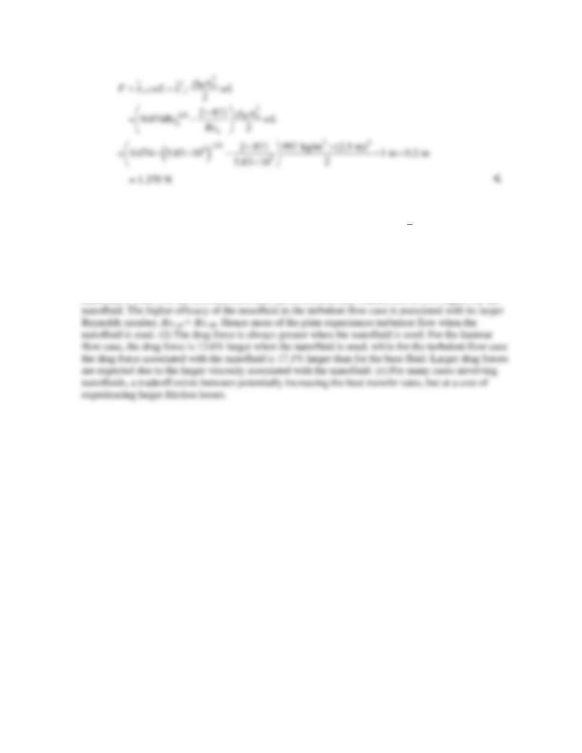
(c) For water flowing over the plate at um = 2.5 m/s,
and the convection heat transfer rate from the top of the plate is
The drag force on the plate is
Continued…
PROBLEM 7.26 (Cont.)
where Equation 7.40 has been used to determine the average friction coefficient.
(d) For the nanofluid flowing over the plate at um = 2.5 m/s, ReL = 5.96 105,
L
h
= 4024 W/m2K, q =
8050 W = 8.05 kW, and F = 1.615 N. <
COMMENTS: (1) The convection heat transfer rate is greater for the nanofluid than for the base
fluid (water). For the laminar case, the nanofluid convection heat transfer rate is 9.5% larger when the
nanofluid is used. For the turbulent flow case the convection heat transfer rate is 13% higher for the
PROBLEM 7.27
KNOWN: Operating power of electrical components attached to one side of copper plate. Contact
resistance. Velocity and temperature of water flow on opposite side.
FIND: (a) Plate temperature, (b) Component temperature.
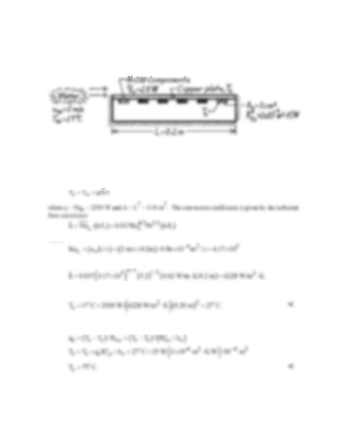
SCHEMATIC:
ASSUMPTIONS: (1) Steady-state conditions, (2) Constant properties, (3) Negligible heat loss from
sides and bottom, (4) Turbulent flow throughout.
PROPERTIES: Water (given): = 0.96 10–6 m2/s, k = 0.620 W/mK, Pr = 5.2.
ANALYSIS: (a) From the convection rate equation,
where
and hence
The plate temperature is then
(b) For an individual component, a rate equation involving the component’s contact resistance can be
used to find its temperature,
COMMENTS: With
5
L
Re 4.17 10 ,
the boundary layer would be laminar over the entire plate
without the boundary layer trip, causing Ts and Tc to be appreciably larger.
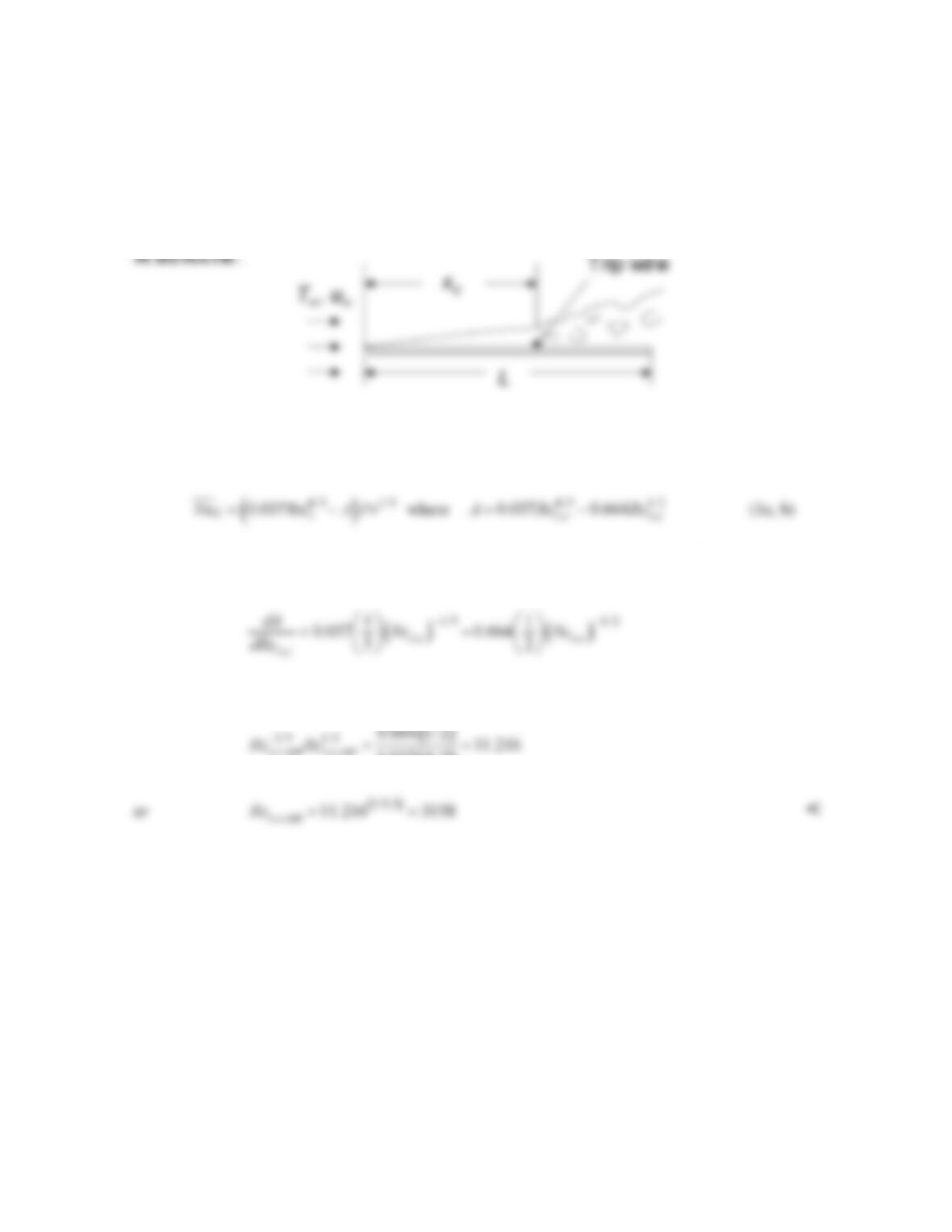
PROBLEM 7.28
KNOWN: Length of isothermal flat plate in parallel flow, L.
FIND: Expression for the Reynolds number associated with the location of a trip wire to maximize
heat transfer, Rex,c,opt.
ASSUMPTIONS: (1) Constant properties.
ANALYSIS: From Equations 7.38 and 7.39
To maximize the average Nusselt number, it is necessary to minimize the value of A. Taking the
derivative of A with respect to Rex,c results in
Setting dA/dRex,c equal to zero yields
0.037 4 / 5
COMMENTS: Substituting Rex,c,opt = 3158 into Equation 1b yields Aopt = – 14. Since A = 0
corresponds to tripping the boundary layer at the leading edge of the plate, and A = 871 corresponds to
a critical Reynolds number of Rex,c = 5 × 10⁵, we know that placing the trip wire at an x location
corresponding to Rex,c,opt = 3158 must maximize heat transfer from the plate (as opposed to
minimizing heat transfer from the plate).
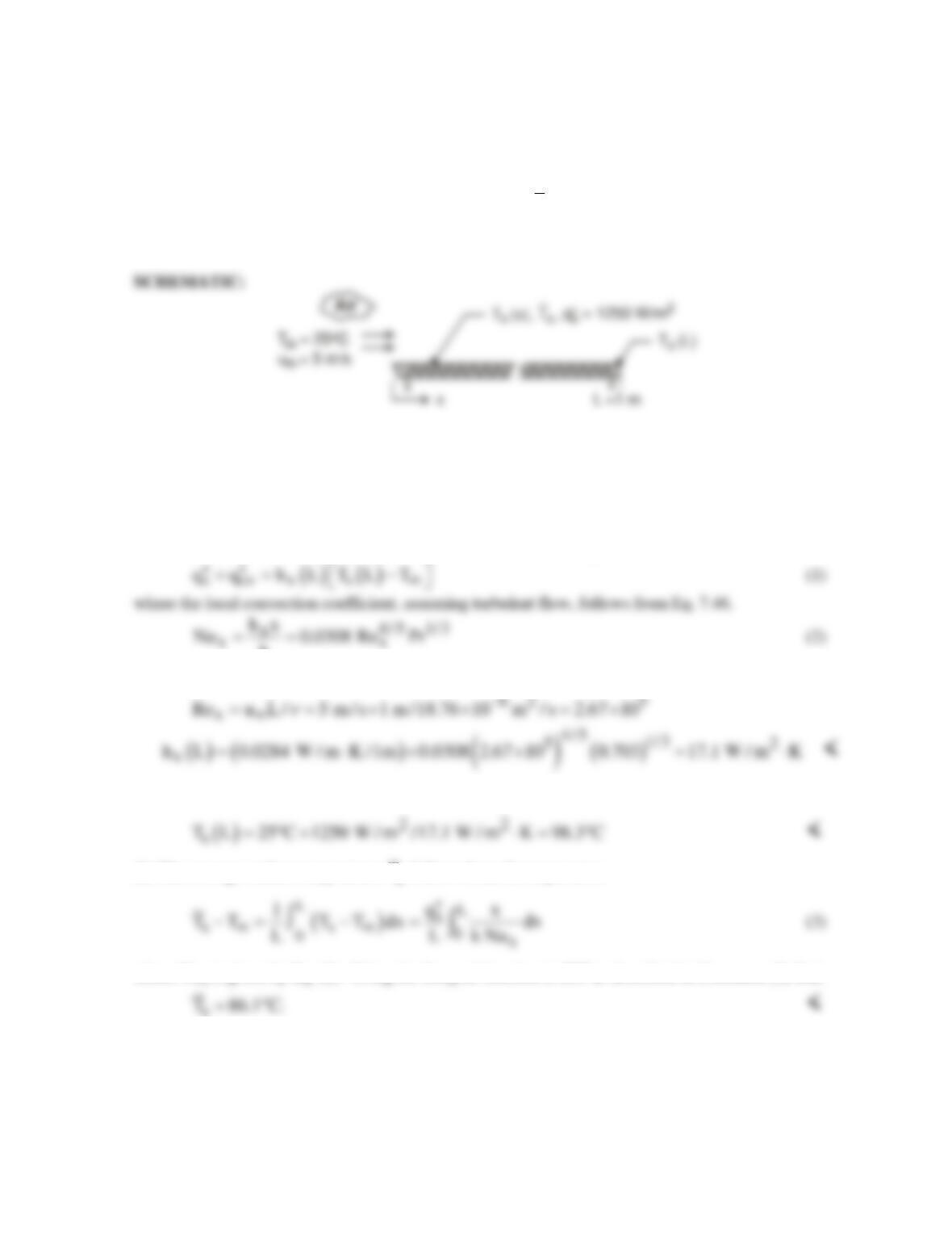
PROBLEM 7.29
KNOWN: Air at atmospheric pressure and a temperature of 25C in parallel flow at a velocity of 5
m/s over a 1-m long flat plate with a uniform heat flux of 1250 W/m2.
FIND: (a) Plate surface temperature, Ts(L), and local convection coefficient, hx(L), at the trailing
edge, x = L, (b) Average temperature of the plate surface,
s
T,
(c) Plot the variation of the plate surface
temperature, Ts(x), and the convection coefficient, hx(x), with distance on the same graph; explain key
features of these distributions.
ASSUMPTIONS: (1) Steady-state conditions, (2) Flow is fully turbulent, and (3) Constant
properties.
PROPERTIES: Table A-4, Air (assume Tf = 325 K, 1 atm): = 18.76 10-6 m2/s; k = 0.0284
W/mK; Pr = 0.703.
ANALYSIS: (a) At the trailing edge, x = L, the convection rate equation is
k
With x = L = 1m, find
Substituting numerical values into Eq. (1),
(b) The average surface temperature
s
T
follows from the expression
where Nux is given by Eq. (2). Using the Integral function in IHT as described in Comment (3) find
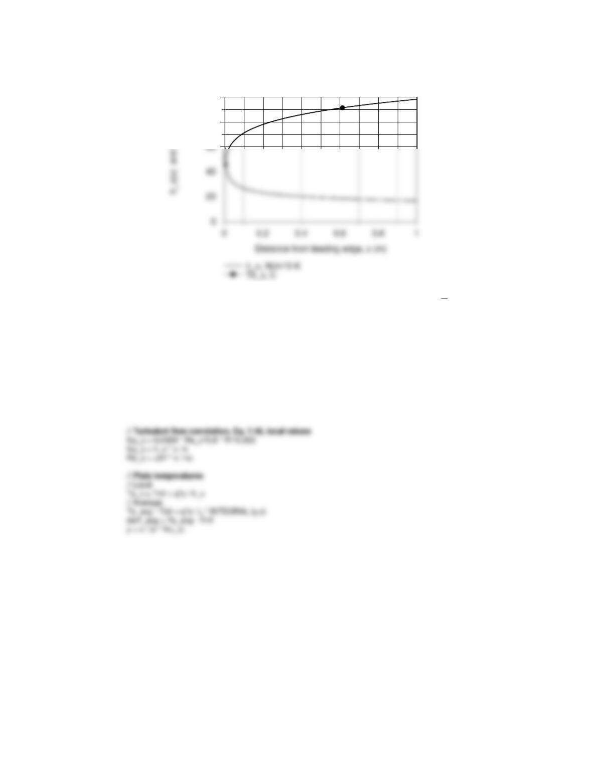
(c) The variation of the plate surface temperature Ts(x) and convection coefficient, hx(x), shown in the
graph are calculated using Eqs. (1) and (2).
Continued …
PROBLEM 7.29 (Cont.)
80
100
COMMENTS: (1) The properties for the correlation should be evaluated at
fs
T T T / 2.
From the foregoing analyses, Tf = (86.1 + 25)/2 = 55.5C = 329 K. Hence, the assumed value of 325
K was reasonable.
(2) The IHT code, excluding the input variables and air property functions, used to evaluate the
integral of Eq. (3) and generate the graphs in part (c) is shown below.
/* Programming note: when using the INTEGRAL function, the value of the independent variable
must not be specified as an input variable. If done so, this error message will appear:
“Redefinition of a constant variable.” */
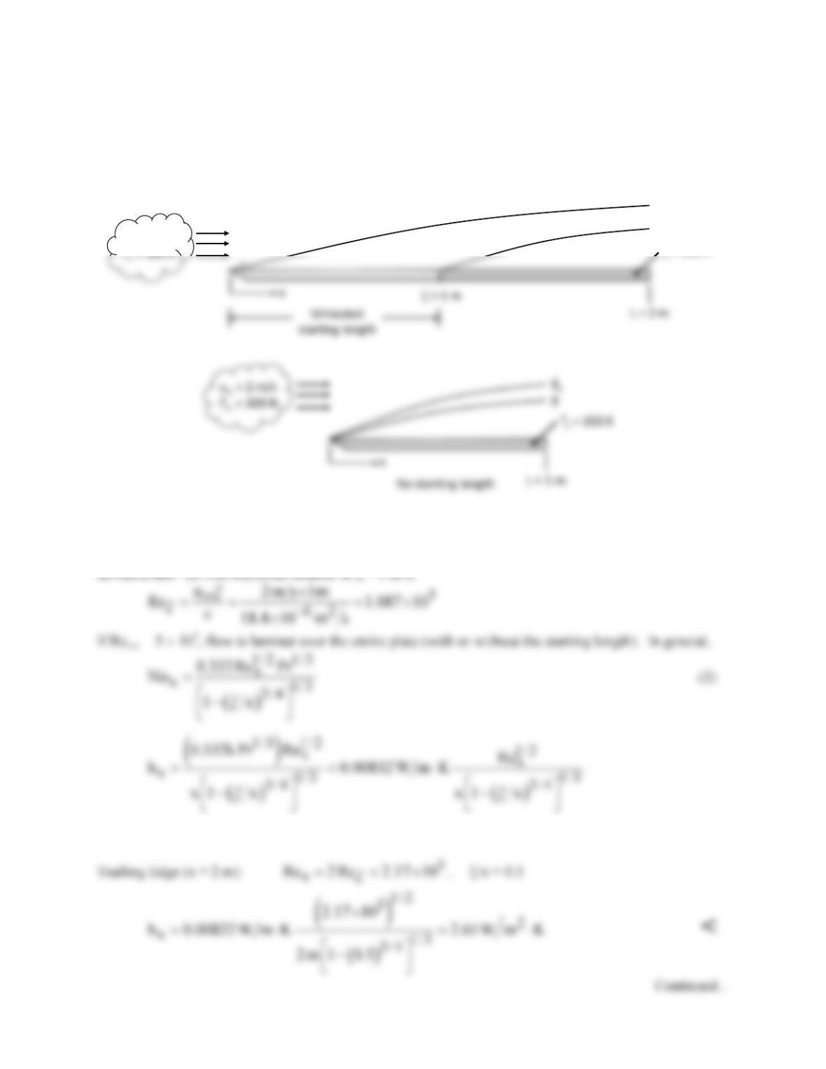
PROBLEM 7.30
KNOWN: Conditions for airflow over isothermal plate with optional unheated starting length.
FIND: (a) local coefficient, hx, at leading and trailing edges with and without an unheated starting
length, ξ = 1 m, (b) average convection coefficient for same conditions, (c) variation of local convection
coefficient over plate with and without unheated starting length.
SCHEMATIC:
δt
δ
u= 2 m/s
PROPERTIES: Table A.4, Air (Tf = 325 K, 1 atm): = 18.4 10-6 m2/s, Pr = 0.703, k = 0.0282
W/mK.
With Unheated Starting Length: Leading edge (x = 1 m): Rex = Reξ, ξ/x = 1, hx = <
PROBLEM 7.30 (Cont.)
Without Unheated Starting Length: Leading edge (x = 0): hx = <
(b) The average convection coefficient
L
h
for the two cases in the schematic are, from Eq. 6.14,
<
(c) The variation of the local convection coefficient over the plate, with and without the unheated starting
length, using Eq. (1) is shown below. The abscissa is x – ξ.
20
COMMENTS: (1) When the velocity and thermal boundary layers grow simultaneously (without
starting length), we expect the local and average coefficients to be larger than when the velocity
boundary layer is thicker (with starting length).
h
h
L
L
L
(3) The numerical integration of Eq. (2) was performed using the INTEGRAL (f,x) operation in IHT as
shown in the Workspace below.

PROBLEM 7.30 (Cont.)
// Properties Tool – Air:
// Air property functions : From Table A.4
// Units: T(K); 1 atm pressure
PROBLEM 7.31
KNOWN: Cover plate dimensions and temperature for flat plate solar collector. Air flow conditions.
FIND: (a) Heat loss with simultaneous velocity and thermal boundary layer development, (b) Heat
loss with unheated starting length.
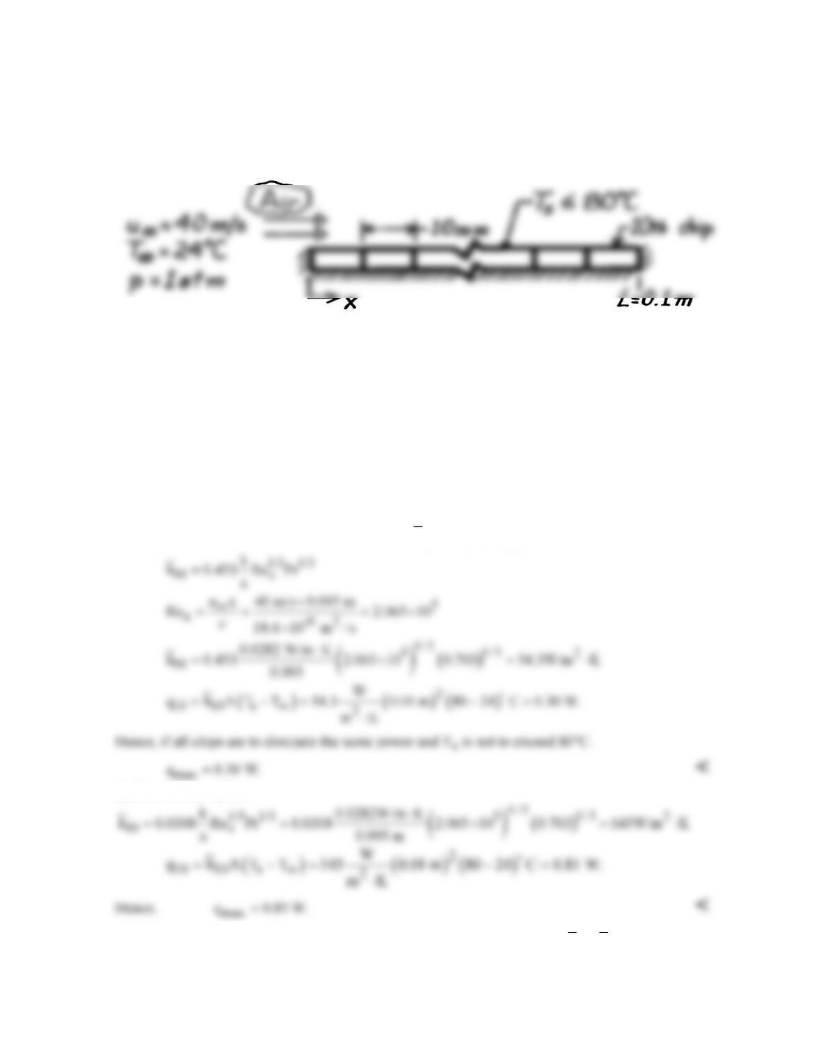
SCHEMATIC:
ASSUMPTIONS: (1) Steady-state conditions, (2) Negligible radiation, (3) Boundary layer is not
disturbed by roof-plate interface, (4)
5
x,c
Re 5 10 .
PROPERTIES: Table A-4, Air (Tf = 285.5K, 1 atm): = 14.6 10-6 m2/s, k = 0.0251 W/mK, Pr
= 0.71.
ANALYSIS: (a) The Reynolds number for the plate of L = 1m is
For laminar flow
L
L 1m
(b) The Reynolds number for the roof and collector of length L = 3m is
Hence, laminar boundary layer conditions exist throughout and the heat rate is
Using a numerical technique to evaluate the integral,
COMMENTS: Values of
h
with and without the unheated starting length are 3.9 and 5.5 W/m2K.
Prior development of the velocity boundary layer decreases
h.
PROBLEM 7.32
KNOWN: Surface dimensions for an array of 10 silicon chips. Maximum allowable chip
temperature. Air flow conditions.
FIND: Maximum allowable chip electrical power (a) without and (b) with a turbulence promoter at
the leading edge.
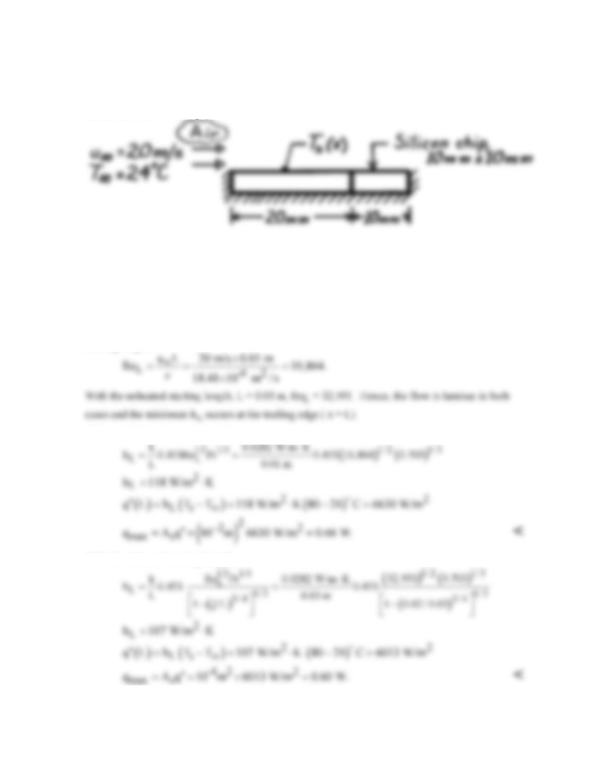
SCHEMATIC:
ASSUMPTIONS: (1) Steady-state conditions, (2) Film temperature of 52C, (3) Negligible
radiation, (4) Negligible heat loss through insulation, (5) Uniform heat flux at chip interface with air,
(6)
5
x,c
Re 5 10 .
PROPERTIES: Table A-4, Air (Tf = 325K, 1 atm): = 18.4 10-6 m2/s, k = 0.0282 W/mK, Pr =
0.703.
ANALYSIS:
-6 2 5
L
Re u L/ 40 m/s 0.1 m/18.4 10 m / s 2.174 10 .
Hence, flow is
laminar over all chips without the promoter.
(a) For laminar flow, the minimum hx exists on the last chip. Approximating the average coefficient
for Chip 10 as the local coefficient at x = 95 mm,
10 x 0.095m
hh .
(b) For turbulent flow,
COMMENTS: It is far better to orient array normal to the air flow. Since
h h
1 10
>,
more heat
could be dissipated per chip, and the same heat could be dissipated from each chip.
PROBLEM 7.33
KNOWN: Dimensions and maximum allowable temperature of a silicon chip. Air flow conditions.
FIND: Maximum allowable power with or without unheated starting length.
SCHEMATIC:
ASSUMPTIONS: (1) Steady-state conditions, (2) Tf = 52C, (3) Negligible radiation, (4) Negligible
heat loss through insulation, (5) Uniform heat flux at chip-air interface, (6) Rex,c = 5 105.
PROPERTIES: Table A-4, Air (Tf = 325K, 1 atm): = 18.41 10-6 m2/s, k = 0.0282 W/mK, Pr =
0.703.
ANALYSIS: For uniform heat flux, maximum Ts corresponds to minimum hx. Without unheated
starting length,
Without unheated starting length,
With the unheated starting length,
COMMENTS: Prior velocity boundary layer development on the unheated starting section decreases
hx, although the effect diminishes with increasing x.
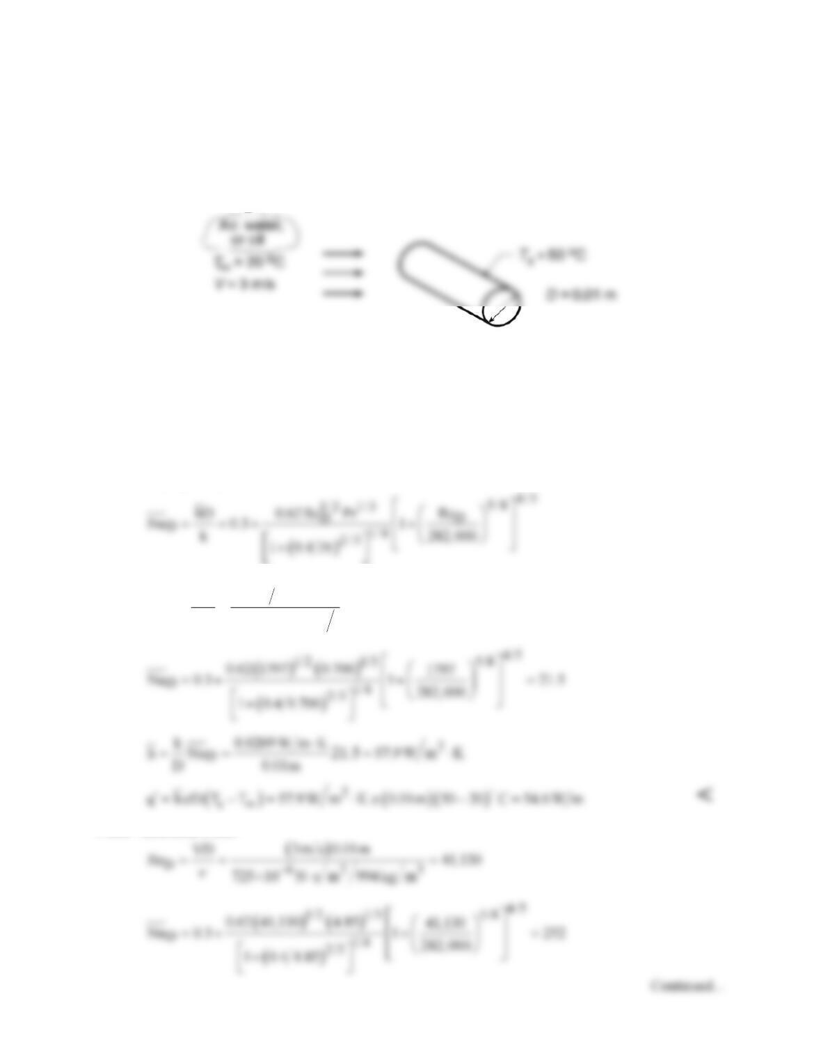
PROBLEM 7.34
KNOWN: Cylinder diameter and surface temperature. Temperature and velocity of fluids in cross flow.
FIND: (a) Rate of heat transfer per unit length for the fluids: atmospheric air and saturated water, and
engine oil, for velocity V = 3 m/s, using the Churchill-Bernstein correlation, and (b) Compute and plot
q′
as a function of the fluid velocity 0.5 ≤ V ≤ 10 m/s.
SCHEMATIC:
ASSUMPTIONS: (1) Steady-state conditions, (2) Uniform cylinder surface temperature.
PROPERTIES: Table A.4, Air (Tf = 308 K, 1 atm): = 16.69 10-6 m2/s, k = 0.0269 W/mK, Pr =
0.706; Table A.6, Saturated Water (Tf = 308 K): = 994 kg/m3, µ = 725 10-6 Ns/m2, k = 0.625
W/mK, Pr = 4.85; Table A.5, Engine Oil (Tf = 308 K): = 340 10-6 m2/s, k = 0.145 W/mK, Pr =
4000.
ANALYSIS: (a) For each fluid, calculate the Reynolds number and use the Churchill-Bernstein
correlation, Eq. 7.54,
Fluid: Atmospheric Air
D62
3m s 0.01m
VD
Re 1797
16.69 10 m s
Fluid: Saturated Water
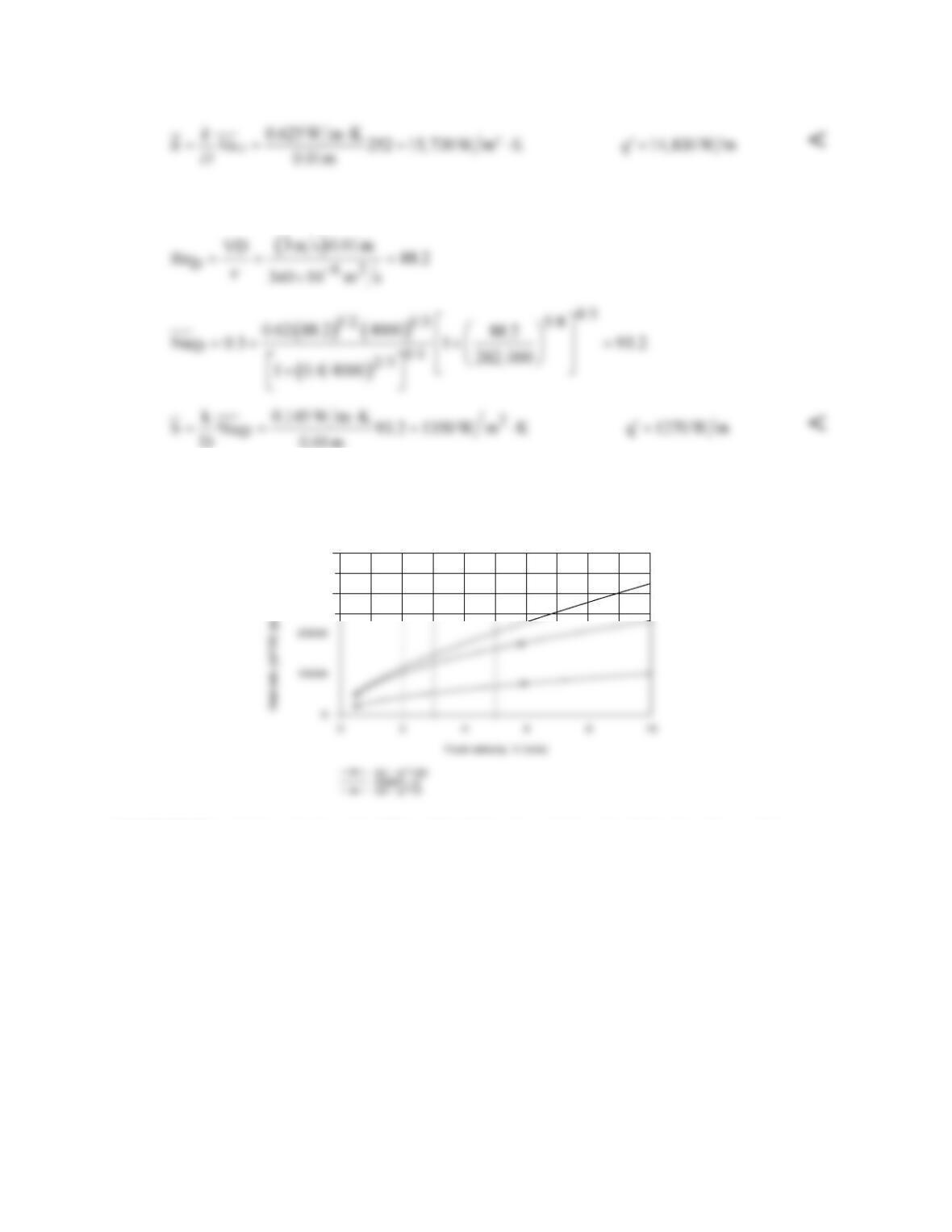
PROBLEM 7.34 (Cont.)
Fluid: Engine Oil
D 0.01m
(b) Using the IHT Correlations Tool, External Flow, Cylinder, along with the Properties Tool for each
of the fluids, the heat rates,
q′
, were calculated for the range 0.5 ≤ V ≤ 10 m/s. Note the
q′
scale
multipliers for the air and oil fluids which permit easy comparison of the three curves.
30000
40000
COMMENTS: (1) Note the inapplicability of the Zukauskas relation, Eq. 7.53, since Proil > 500.
(2) In the plot above, recognize that the heat rate for the water is more than 10 times that with oil and 300
times that with air. How do changes in the velocity affect the heat rates for each of the fluids?
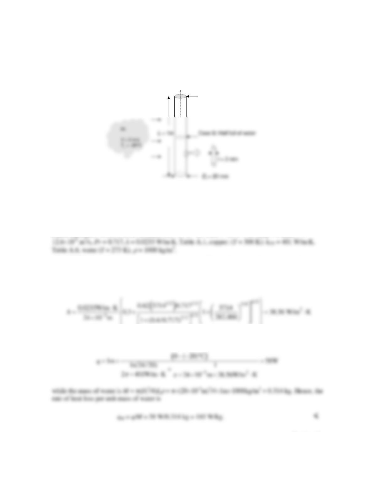
PROBLEM 7.35
KNOWN: Dimensions of a vertical copper tube experiencing crossflow. Air velocity and
temperature, water temperature inside the tube.
FIND: (a) The rate of heat loss per unit mass from the water (W/kg) when the pipe is full. (b) The rate
of heat loss from the water (W/kg) when the pipe is half full.
SCHEMATIC:
ASSUMPTIONS: (1) Steady-state conditions, (2) Constant properties, (3) Tube behaves as an
infinite fin, (4) Water is well-mixed, (5) One-dimensional heat transfer, (6) Inside copper wall
temperature at water temperature, (7) Negligible heat transfer to/from the gas above the liquid water,
(8) Negligible radiation.
PROPERTIES: Table A.4, air assumed: (Tf = (0C – 20C)/2 = -10C 263K, p = 1 atm):
=
ANALYSIS: For either case, the average convection coefficient about the tube must be evaluated.
The Reynolds number, based upon the outer diameter Do = 20 mm + 4 mm = 24 mm is ReD = VDo/
=
3 m/s 24 10-3 m/12.6 10-6 m2/s = 5714. Using Eq. 7.54, the average heat transfer coefficient
about the exterior of the tube is
(a) From Eq. 3.34 the rate of heat loss from the water is
Continued…
Case A: Full of water