Chapter 7 the other must be its complex conjugate

Chapter 7

7.4.49 The matrix of Twith respect to the standard basis 1, x, x2is B=



1−1 1

0 3 −6



. The eigenvalues of Bare

7.4.50 The matrix of Twith respect to the standard basis 1, x, x2is B=



1−3 9

0 1 −6

001



. The only eigenvalue of B



7.4.51 The nonzero constant functions f(x) = bare the eigenfunctions with eigenvalue 0. If f(x) is a polynomial

of degree ≥1, then the degree of f(x) exceeds the degree of f′(x) by 1 (by the power rule of calculus), so that

f′(x) cannot be a scalar multiple of f(x). Thus 0 is the only eigenvalue of T, and the eigenspace E0consists of

the constant functions.

7.4.53 In Exercises 7.2.30, 7.2.31, and 7.3.32, we prove the following facts concerning the eigenvalues of a positive

transition matrix B:

1. λ= 1 is an eigenvalue of Bwith gemu(1) = 1.

2. If λis any eigenvalue of B, then −1< λ ≤1.

7.4.54 Note that A2= 0, but B26= 0. Since A2fails to be similar to B2, matrix Aisn’t similar to B(see Example

7 of Section 3.4).

350

Section 7.4

7.4.56 The hint shows that matrix M=AB 0

B0is similar to N=0 0

B BA ; thus matrices Mand Nhave the

7.4.57 Modifying the hint in Exercise 56 slightly, we can write AB 0

B0ImA

0In=ImA

0In

0 0

B BA . Thus matrix M=AB 0

B0is similar to N=0 0

B BA . By Theorem 7.3.5a, matrices M

and Nhave the same characteristic polynomial.

7.4.58 a. If ~v is in the image of A, then ~v =A ~w for some vector ~w. Now A~v =A2~w =~

0, showing that ~v is in the

kernel of A.

b. From part (a) we know that dim imA≤dim ker A. Also, dim imA > 0 since Ais nonzero, and dim ker A+

dim imA= 3 by the rank-nullity theorem. This leaves us with only one possibility, namely, dim imA= 1 and

dim ker A= 2.

7.4.59 Yes, Ais similar to B, since both Aand Bare similar to 



010

000



, by Exercise 58.

Chapter 7

7.4.60 We will use the method outlined in Exercise 58. We start with the vector ~v1=



1

2

3



in the image of A.

7.4.61 First we need to verify that the vectors ~v1, …, ~vr, ~w1, …, ~wr, ~u1, …, ~umare linearly independent. Consider a

relation a1~v1+… +ar~vr+b1~w1+… +br~wr+c1~u1+… +cm~um=~

0. Multiplying both sides with A, we find

b1~v1+… +br~vr=~

0, so that b1=… =br= 0 since the ~viare independent by construction. Now the aiand the

7.4.62 A nonzero function fis an eigenfunction of Twith eigenvalue λif T(f) = f′′ +af ′+bf =λf, or, f′′ +af′+

(b−λ)f= 0. By Theorem 4.1.7, this differential equation has a two-dimensional solution space. Thus all real

numbers are eigenvalues of T, and all the eigenspaces are two-dimensional.

7.4.63 a We need to solve the differential equation f′′(x) = f(x). As in Example 18 of Section 4.1, we will look for

exponential solutions. The function f(x) = ekx is a solution if k2= 1, or k=±1. Thus the eigenspace E1is the

span of functions exand e−x.

7.4.64 The eigenvalues of Aare 1 and 3, with associated eigenvectors 1

7.4.65 Let’s write Sin terms of its columns, as S= [ ~v ~w ].

We want A[~v ~w ] = [ ~v ~w ]5 0

0−1,or, [ A~v A ~w ] = [ 5~v −~w ],that is, we want ~v to be in the eigenspace

Section 7.4

7.4.66 For Awe find the eigenspaces E1= span 





1

0



,



0

1

−1





and E2= span 





1

0





. If we write S= [~u ~v ~w],

7.4.67 Let Eλ1= span(~v1, ~v2, ~v3) and Eλ2= span( ~w1, ~w2). As in Exercise 65, we can see that Smust be of the

form [ ~x1~x2~x3~x4~x5] where ~x1, ~x2and ~x3are in Eλ1and ~x4and ~x5are in Eλ2. Thus, we can write

~x1=c1~v1+c2~v2+c3~v3,for example, or ~x5=d1~w1+d2~w2.

Using Summary 4.1.6, we find a basis: [ ~v1~

0~

0 ] ,[~v2~

0~

0 ] ,

7.4.68 Let ~v1, . . . , ~vnbe an eigenbasis for A, with A~vi=λi~vi. Arguing as in Exercises 64 through 67, we see that

the ith column of Smust be in Eλi,so that it must be of the form ci~vifor some scalar ci. The matrices Swe

seek are of the form S= [c1~v1. . . cn~vn],involving the narbitrary constants c1, . . . , cn,so that the dimension of

Vis n.

7.4.69 aBis diagonalizable since it has three distinct eigenvalues, so that S−1BS is diagonal for some invertible S.

But S−1AS =S−1I3S=I3is diagonal as well. Thus Aand Bare indeed simultaneously diagonalizable.

353

Chapter 7

7.4.70 Consider an n×nmatrix Awith mdistinct eigenvalues λ1, …, λm.

If ~v is an eigenvector of Awith eigenvalue λm, then (A−λmIn)~v =~

0, so that

(A−λ1In) (A−λ2In)· · · (A−λmIn)~v =~

0. Since the factors in the product

7.3.3b.

7.4.71 The eigenvalues are 1 and 2, and (A−I3) (A−2I3) = 0. Thus Ais diagonalizable.

7.4.73 If an n×nmatrix Ahas mdistinct eigenvalues λ1, …, λm, then we can write its characteristic polynomial

as fA(λ) = (λ−λ1) (λ−λ2)· · · (λ−λm)g(λ) for some polynomial g(λ) of degree n−m. Now fA(A) =

7.4.74 a For a diagonalizable n×nmatrix Awith only two distinct eigenvalues, λ1and λ2, we have (A−λ1In)(A−

λ2In) = 0, by Exercise 70. Thus the column vectors of A−λ2Inare in the kernel of A−λ1In,that is, they

are eigenvectors of Awith eigenvalue λ1(or else they are ~

0). Conversely, the column vectors of A−λ1Inare

eigenvectors of Awith eigenvalue λ2(or else they are ~

0).

b If Ais a 2 ×2 matrix with distinct eigenvalues λ1and λ2,then the nonzero columns of A−λ1I2are eigenvectors

Section 7.5

7.5.1z= 3 −3iso |z|=p32+ (−3)2=√18 and arg(z) = −π

4,

so z=√18 cos −π

4+isin −π

4.

354

Section 7.5

7.5.2If z=r(cos θ+isin θ) then z4=r4(cos 4θ+isin 4θ).

7.5.3If z=r(cos θ+isin θ), then zn=rn(cos(nθ) + isin(nθ)).

zn= 1 if r= 1,cos(nθ) = 1,sin(nθ) = 0 so nθ = 2kπ for an integer k, and θ=2kπ

n,

7.5.4Let z=r(cos θ+isin θ) then w=√rcos θ+2πk

2+isin θ+2πk

2,k= 0, 1.

7.5.5Let z=r(cos θ+isin θ) then w=n

√rcos θ+2πk

n+isin θ+2πk

n,k= 0,1,2,…,n−1.

355

Chapter 7

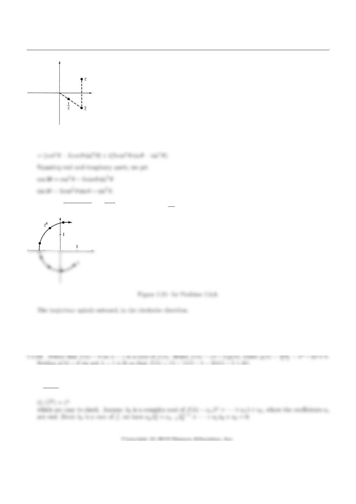
Figure 7.26: for Problem 7.5.6.

7.5.9|z|=√0.82+ 0.72=√1.15, arg(z) = arctan −0.7

0.8≈ −0.72. See Figure 7.27.

7.5.10 Let p(x) = ax3+bx2+cx +d, where a6= 0. Since pmust have a real root, say λ1, we can write p(x) =

a(x−λ1)g(x) where g(x) is of the form g(x) = x2+px +q. On page 367, we see that g(x) = (x−λ2)(x−λ3),

so that p(x) = a(x−λ1)(x−λ2)(x−λ3), as claimed.

7.5.12 We will use the facts:

i) z+w= ¯z+ ¯wand

356

Section 7.5

7.5.13 2i

1=0

1

|{z }

~v

+i2

0

|{z }

~w

is an eigenvector with eigenvalue 2i, so that we can let S=~w ~v =2 0

0 1 ,

with S−1AS =0−2

2 0 .

7.5.16 1

1 + i=1

1

|{z }

~v

+i0

1

|{z }

~w

is an eigenvector with eigenvalue 4 + i, so that we can let S=~w ~v =

0 1

1 1 , with S−1AS =4−1

1 4 .

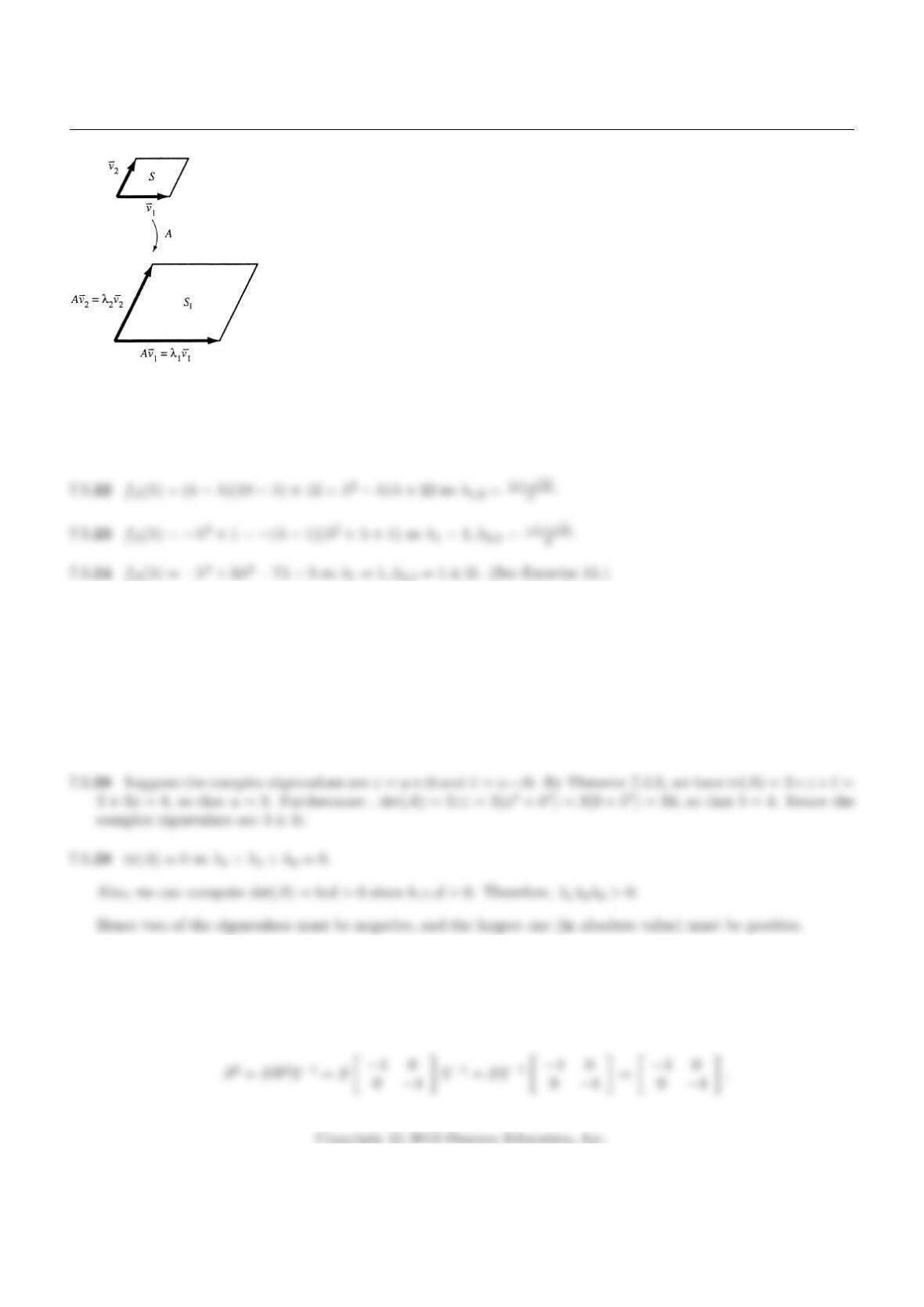
7.5.18 Let ~v1, ~v2be two eigenvectors of A. They define a parallelogram of area S=|det[~v1~v2]|. Now A~v1=λ1~v1and

A~v2=λ2~v2define a parallelogram of area S1=|det[λ1~v1λ2~v2]|=|λ1λ2det[~v1~v2]|so S1

S=|λ1λ2|=|det(A)|.

Hence |det(A)|=|λ1λ2|, as claimed. In R3, a similar argument holds if we replace areas by volumes. See Figure

7.28.

7.5.19 a Since Ahas eigenvalues 1 and 0 associated with Vand V⊥respectively and since Vis the eigenspace of

λ= 1, by Theorem 7.5.5, tr(A) = m, det(A) = 0.

357

Chapter 7

Figure 7.28: for Problem 7.5.18.

7.5.21 fA(λ) = (11 −λ)(−7−λ) + 90 = λ2−4λ+ 13 so λ1,2= 2 ±3i.

7.5.25 fA(λ) = λ4−1 = (λ2−1)(λ2+ 1) = (λ−1)(λ+ 1)(λ−i)(λ+i) so λ1,2=±1 and λ3,4=±i

7.5.26 fA(λ) = (λ2−2λ+ 2)(λ2−2λ) = (λ2−2λ+ 2)(λ−2)λ= 0, so λ1,2= 1 ±i, λ3= 2, λ4= 0.

7.5.27 By Theorem 7.5.5, tr(A) = λ1+λ2+λ3, det(A) = λ1λ2λ3but λ1=λ26=λ3by assumption, so tr(A) = 1 =

2λ2+λ3and det(A) = 3 = λ2

2λ3.

Solving for λ2, λ3we get −1,3 hence λ1=λ2=−1 and λ3= 3. (Note that the eigenvalues must be real; why?)

7.5.30 a. The eigenvalues of a 2 ×2 matrix are the roots of a quadratic equation. Since one of the eigenvalues of

Ais 2i, the other must be its complex conjugate, −2i. Now Ais similar to B=2i0

0−2i, meaning that

A=SBS−1for some invertible Swith complex entries. We find

358

Section 7.5

7.5.31 a. Computing A20, we conjecture that

lim

t→∞ At=1

5







1 1 1 1 1







1

d. We can adapt the proof of Theorem 7.4.1; see the second paragraph on Page 350 in particular. Since Ais

diagonalizable over the complex numbers, there exists a complex eigenbasis ~v1, ~v2, …, ~v5for A, where A~vi=λi~vi,

with the eigenvalues λiwe found in part b. Note that λ1= 1 and |λi|<1 for i= 2,3,4,5. If ~x0=c1~v1+c2~v2+

… +c5~v5, then At~x0=c1~v1+c2λt

7.5.32 a. Computing A20, we conjecture that

lim

t→∞ At=



0.36 0.36 0.36

0.26 0.26 0.26

0.38 0.38 0.38





359

Chapter 7

7.5.33 aCis obtained from Bby dividing each column of Bby its first component. Thus, the first row of Cwill

consist of 1’s.

b We observe that the columns of Care almost identical, so that the columns of Bare “almost parallel” (that is,

almost scalar multiples of each other).

7.5.34 a The eigenvalues of A−λInare λ1−λ, λ2−λ, . . . , λn−λ, and we were told that |λ1−λ|<|λi−λ|for

i= 2,…,n. We may assume that λ16=λ(otherwise we are done).

The eigenvalues of (A−λIn)−1are (λ1−λ)−1,(λ2−λ)−1,…,(λn−λ)−1, and (λ1−λ)−1has the largest modulus.

The matrices A, A −λIn, and (A−λIn)−1have the same eigenvectors.

For large t, the columns of the tth power of (A−λIn)−1will be almost eigenvectors of A. If ~v is such a column,

compare ~v and A~v to find an approximation of λ1.

360

Section 7.5

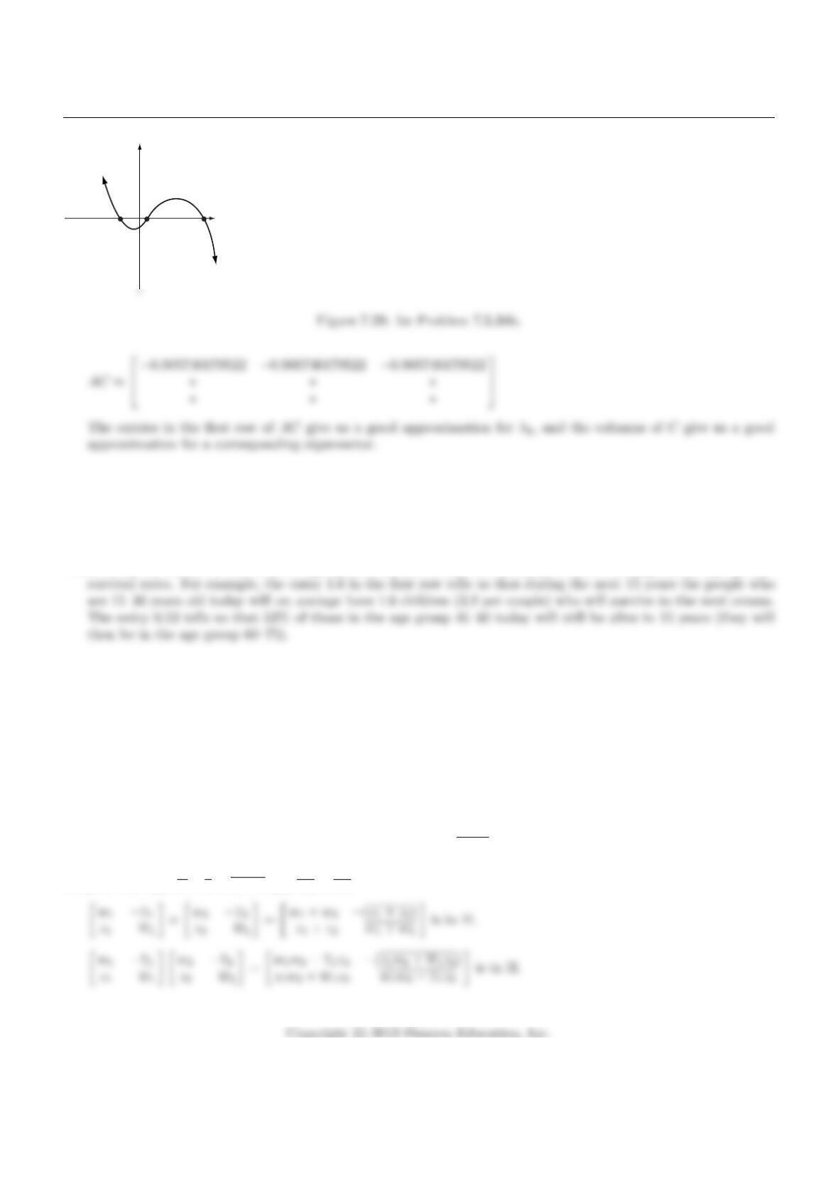
λ1≈ −1 λ2≈ 0

λ3≈ 17

(not to scale)

7.5.35 We have fA(λ) = (λ1−λ)(λ2−λ)···(λn−λ)

= (−λ)n+ (λ1+λ2+···+λn)(−λ)n−1+···+ (λ1λ2···λn). But, by Theorem 7.2.5, the coefficient of (−λ)n−1

is tr(A). So, tr(A) = λ1+···+λn.

7.5.36 a The entries in the first row are age-specific birth rates and the entries just below the diagonal are age-specific

b Using technology, we find the largest eigenvalue λ1= 1.908 with associated eigenvector

~v1≈







0.574

0.247

0.115

0.047

0.014

0.002







.

The components of ~v1give the distribution of the population among the age groups in the long run, assuming

that current trends continue. λ1gives the factor by which the population will grow in the long run in a period

of 15 years; this translates to an annual growth factor of 15

√1.908 ≈1.044, or an annual growth of about 4.4%.

7.5.37 a Use that w+z=w+zand wz =wz.

361

Chapter 7

b If Ain His nonzero, then det(A) = ww +zz =|w|2+|z|2>0, so that Ais invertible.

7.5.38 aC2

4=





0 0 1 0

0 0 0 1

1 0 0 0

0 1 0 0





, C3

4=





0 1 0 0

0 0 1 0

0 0 0 1

1 0 0 0





, C4

4=I4, then C4+k

4=Ck

4.

Figure 7.30 illustrates how C4acts on the basis vectors ~ei.

7.5.39 Figure 7.31 illustrates how Cnacts on the standard basis vectors ~e1, ~e2, . . . , ~enof Rn.

362

Section 7.5

7.5.39 a Based on Figure 7.31, we see that Ck

ntakes ~eito ~ei+k“modulo n,” that is, if i+kexceeds nthen Ck

ntakes

~eito ~ei+k−n(for k= 1,…,n−1).

7.5.40 In Exercise 7.2.50 we derived the formula x=3

rq

2+qq

22+p

33+3

rq

2−qq

22+p

33

for the solution of the equation x3+px =q. Here q

22+p

33is negative, and we can write

x=3

rq

2+iq−q

22+−p

33+3

rq

2−iq−q

22+−p

33.

Let us write this solution in polar coordinates:

x=3

q−p

33/2(cos α+isin α) + 3

q−p

33/2(cos α−isin α)

=p−p

3cos α+2πk

3+isin α+2πk

3+q−p

3cos α+2πk

3−isin α+2πk

3

= 2p−p

3cos α+2πk

3, k = 0,1,2. See Figure 7.32.

Figure 7.32: for Problem 7.5.40.

3)3/2.

363

Chapter 7

7.5.41 Substitute ρ=1

xinto 14ρ2+ 12ρ3−1 = 0;

14

x2+12

x3−1 = 0

14x+ 12 −x3= 0

x3−14x= 12

Now use the formula derived in Exercise 40 to find x, with p=−14 and q= 12. There is only one positive

solution, x≈4.114, so that ρ=1

x≈0.243.

7.5.43 Note that f(z) is not the zero polynomial, since f(i) = det(S1+iS2) = det(S)6= 0, as Sis invertible. A

nonzero polynomial has only finitely many zeros, so that there is a real number xsuch that f(x) = det(S1+xS2)6=

0, that is, S1+xS2is invertible. Now SB =AS or (S1+iS2)B=A(S1+iS2). Considering the real and the

imaginary part, we can conclude that S1B=AS1and S2B=AS2and therefore (S1+xS2)B=A(S1+xS2).

Since S1+xS2is invertible, we have B= (S1+xS2)−1A(S1+xS2), as claimed.

7.5.44 Let Abe a complex 2 ×2 matrix. Let λbe a complex eigenvalue of A, and consider an associated eigenvector

~v, so that A~v =λ~v. Now let Pbe an invertible 2 ×2 matrix of the form P= [~v ~w] (the first column of Pis

our eigenvector ~v). Then P−1AP will be of the form λ∗

0∗, so that we have found an upper triangular matrix

similar to A(compare with the proof of Theorem 7.1.3).