Chapter 7
7.2.46 aλ2
1+λ2
2= (λ1+λ2)2−2λ1λ2= (trA)2−2 det(A) = (a+d)2−2(ad −bc) = a2+d2+ 2bc.
7.2.47 Let M= [ ~v1~v2].We want A[~v1~v2] = [ ~v1~v2]2 0
0 3 ,or, [ A~v1A~v2] = [ 2~v13~v2].Since ~v1or ~v2
must be nonzero, 2 or 3 must be an eigenvalue of A.
one real root.
b If v3−u3= 20 and vu = 2 then
(v−u)3+ 6(v−u) = v3−3v2u+ 3vu2−u3+ 6(v−u) = v3−u3−3vu(v−u) + 6(v−u)
Now u3=v3−20 = −10 ±√108 and u=3
d Let v=3
rq
2+qq
22+p
33and u=3
r−q
2+qq
22+p
33.
qq
Section 7.3
Section 7.3
7.3.1λ1= 7, λ2= 9, E7= ker 0 8
0 2 = span 1
0, E9= ker −2 8
0 0 = span 4
1
7.3.2λ1= 2, λ2= 0, E2= span 1
1, E0= span −1
1
7.3.3λ1= 4, λ2= 9, E4= span 3
−2,E9= span 1
1
7.3.6λ1,2=7±√57
2
7.3.7λ1= 1, λ2= 2, λ3= 3, eigenbasis: ~e1,~e2,~e3
We can diagonalize the diagonal matrix Awith S=I3and B=A.
Chapter 7
7.3.8λ1= 1, λ2= 2, λ3= 3, eigenbasis:
1
0
0
,
1
1
0
,
1
2
1
We can diagonalize Awith S=
1 1 1
0 1 2
0 0 1
and B=
1 0 0
0 2 0
0 0 3
.
7.3.10 λ1=λ2= 1, λ3= 0, E1= span
1
0
0
, E0= span
0
0
1
No eigenbasis. This matrix fails to be diagonalizable.
7.3.12 λ1=λ2=λ3= 1, E1= span
1
0
0
, no eigenbasis
7.3.13 λ1= 0, λ2= 1, λ3=−1, eigenbasis:
0
1
0
,
1
−3
1
,
1
−1
2
332
Section 7.3
7.3.16 λ1= 0 (no other real eigenvalues), with eigenvector
1
−1
1
7.3.17 λ1=λ2= 0, λ3=λ4= 1
1
0
0
0
7.3.18 λ1=λ2= 0, λ3=λ4= 1, E0= span(~e1,~e3), E1= span(~e2)
No eigenbasis. This matrix fails to be diagonalizable.
7.3.19 Fails to be diagonalizable. The eigenvalues are 1,0,1, and the eigenspace E1= ker(A−I3)
= span(~e1) is only one-dimensional.
7.3.22 We want Asuch that A~e1= 7~e1and A~e2= 7~e2hence A=7 0
0 7 .
333
Chapter 7
7.3.23 λ1=λ2= 1 and E1= span(~e1), hence there is no eigenbasis. The matrix represents a shear parallel to the
x-axis.
7.3.24 Let A=a b
c d . First we want a b
c d 2
1=2
1,or 2a+b= 2,2c+d= 1. This condition is satisfied
by all matrices of the form A=a2−2a
7.3.25 If λis an eigenvalue of A, then Eλ= ker(A−λI3) = ker
−λ1 0
0−λ1
a b c −λ
.
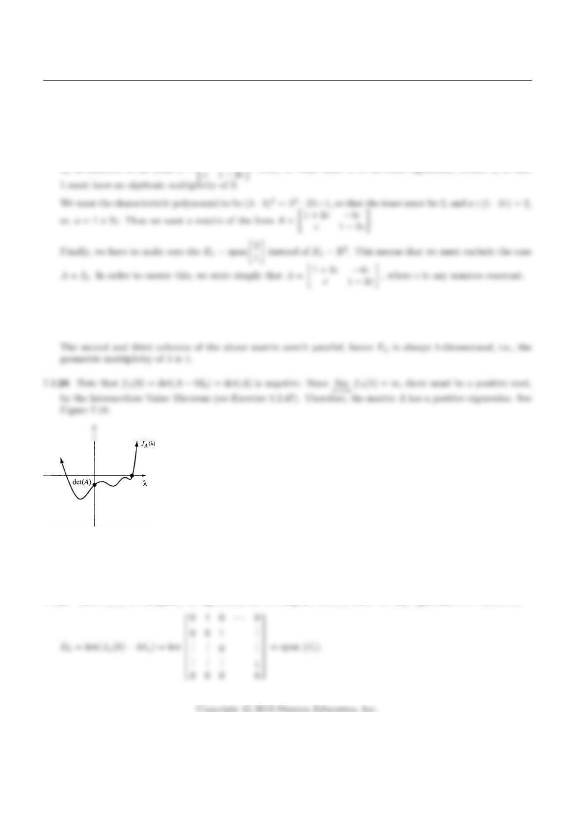
Figure 7.18: for Problem 7.3.26.
7.3.27 By Theorem 7.2.4, we have fA(λ) = λ2−5λ+ 6 = (λ−3)(λ−2) so λ1= 2, λ2= 3.
7.3.28 Since Jn(k) is triangular, its eigenvalues are its diagonal entries, hence its only eigenvalue is k. Moreover,
334
Section 7.3
The geometric multiplicity of kis 1 while its algebraic multiplicity is n.
7.3.29 Note that ris the number of nonzero diagonal entries of A, since the nonzero columns of Aform a basis of
7.3.30 Since Ais triangular, fA(λ) = (a11 −λ)(a22 −λ)···(amm −λ)(0 −λ)n−m.
7.3.32 Recall that a matrix and its transpose have the same rank (Theorem 5.3.9c). The geometric multiplicity of
λas an eigenvalue of Ais dim(ker(A−λIn)) = n−rank(A−λIn).
7.3.33 If S−1AS =B, then
S−1(A−λIn)S=S−1(AS −λS) = S−1AS −λS−1S=B−λIn.
7.3.34 a If ~x is in the kernel of B, then AS~x =SB~x =S~
0 = ~
0, so that S~x is in ker(A).
bTis clearly linear, and the transformation R(~x) = S−1~x is the inverse of T(if ~x is in the kernel of B, then S−1~x
7.3.35 No, since the two matrices have different eigenvalues (see Theorem 7.3.5c).
↑
Asymmetric
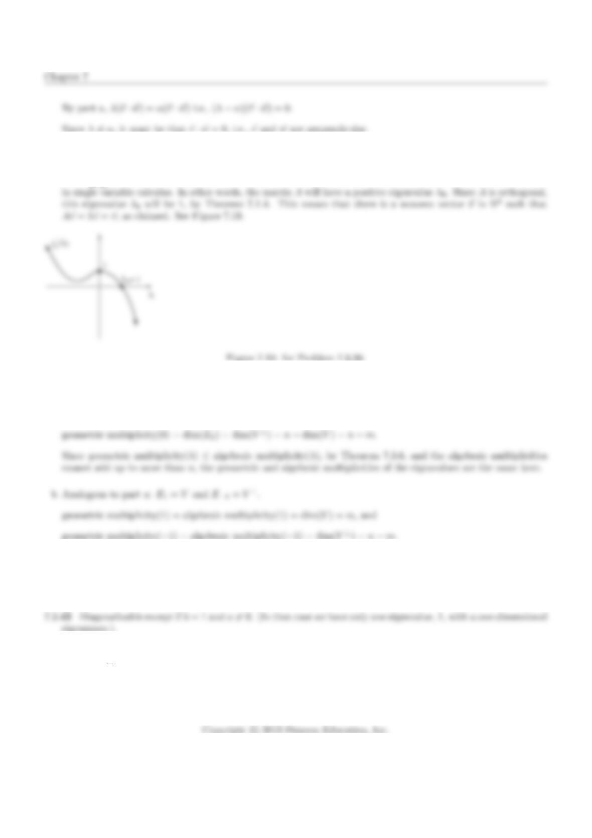
7.3.38 Note that fA(0) = det(A−0I3) = det(A) = 1.
Since lim
λ→∞ fA(λ) = −∞, the polynomial fA(λ) must have a positive root λ0, by the Intermediate Value Theorem
7.3.39 a There are two eigenvalues, λ1= 1 (with E1=V) and λ2= 0 (with E0=V⊥).
Now geometric multiplicity(1) = dim(E1) = dim(V) = m, and
7.3.40 The sole eigenvalue is 1, with algebraic multiplicity 2. This matrix is diagonalizable only if a= 0.
7.3.41 Diagonalizable for all values of a, since there are always two distinct eigenvalues, 1 and 2. See Theorem 7.1.3.
7.3.43 Diagonalizable for positive a. The characteristic polynomial is (λ−1)2−a, so that the eigenvalues are
λ= 1 ±√a. If ais positive, then we have two distinct real eigenvalues, so that the matrix is diagonalizable. If
ais negative, then there are no real eigenvalues. If ais 0, then 1 is the only eigenvalue, with a one-dimensional
eigenspace.
336
Section 7.3
7.3.44 Diagonalizable for all values of a,b, and c. The characteristic polynomial is λ2−(a+c)λ+ac −b2, so that
7.3.45 Diagonalizable for all values of a,b, and c, since we have three distinct eigenvalues, 1, 2, and 3.
7.3.46 The eigenvalues are 1, 2, 1, and the matrix is diagonalizable if (and only if) the eigenspace E1is two-
0a b
0 1 c
7.3.47 Diagonalizable only if a=b=c= 0. Since 1 is the only eigenvalue, it is required that E1=R3, that is, the
matrix must be the identity matrix.
7.3.48 Diagonalizable for positive values of a. The characteristic polynomial is −λ3+aλ =−λ(λ2−a). If ais
7.3.50 First we observe that all the eigenspaces of A=
0 0 a
1 0 3
0 1 0
are one-dimensional, regardless of the value of
a, since rref(A−λI3) is of the form
1 0 ∗
0 1 ∗
0 0 ∗
for all λ. Thus Ais diagonalizable if and only if there are three
7.3.52 The characteristic polynomial is fA(λ) = (−1)nλn−an−1λn−1−… −a1λ−a0. We can prove this by
induction, using Laplace expansion along the first row:
fA(λ) = det (A−λIn) = −λdet (A−λIn)11 + (−1)n+1 a0det (A−λIn)1n
Chapter 7
7.3.53 aB=
0 0 a∗ ∗
1 0 b∗ ∗
0 1 c∗ ∗
0 0 0 ∗ ∗
.
7.3.54 a. B11 =
0 0 0 … 0a0
1 0 0 … 0a1
0 1 0 … 0a2
… … … … … …
,B21 = 0.
d. Our work in parts (a) through (c) shows that fA(A)~v =~
0 for all ~v in Rn, meaning that fA(A) = 0,the zero
matrix.
7.3.55 The non-invertible matrix B=
1 1 1
1 1 1
1 1 1
has 0 as one of its eigenvalues, so that A=B+ 7I3=
8 1 1
1 8 1
1 1 8
has 7 as one of its eigenvalues.
Section 7.4
Section 7.4
7.4.1The eigenvalues of Aare 1 and 3, the diagonal entries of A, and corresponding eigenvectors are 1
0and
1
7.4.2The eigenvalues of Aare 2 and 3, the diagonal entries of A, and corresponding eigenvectors are 1
7.4.3The eigenvalues of Aare -1 and 5, and corresponding eigenvectors are 1
−1and 1
2. Matrix Ais
7.4.4The eigenvalues of Aare 3 and 2, and corresponding eigenvectors are 2
1and 1
1. Matrix Ais diagonal-
Chapter 7
7.4.5The eigenvalues of Aare 0 and 7, and corresponding eigenvectors are 2
−1and 1
3. Matrix Ais
7.4.6The eigenvalues of Aare 0 and 3, and corresponding eigenvectors are 1
−1and 1
2. Matrix Ais
7.4.7The eigenvalues of Aare 0.25 and 1, and corresponding eigenvectors are 1
−1and 1
2. Matrix Ais
7.4.8The eigenvalues of Aare 1 and 0.2, and corresponding eigenvectors are 3
1and 1
−1. Matrix Ais
7.4.9The eigenvalues of Aare 0, -1, and 1, the diagonal entries of the triangular matrix A, and corresponding
eigenvectors are
1
1
,
0
2
and
0
0
. Matrix Ais diagonalizable, with S=
1 0 0
1 2 0
and
340
Section 7.4
7.4.10 The eigenvalues of Aare 1, 0, and 2, the diagonal entries of the triangular matrix A, and corresponding
eigenvectors are
1
0
0
,
1
−1
0
and
3
1
2
. Matrix Ais diagonalizable, with S=
113
0−1 1
002
and B=
7.4.11 We use technology to find that the eigenvalues of Aare 1, 0, and 2, and corresponding eigenvectors are
1
−1
0
,
1
−4
1
and
1
0
−1
. Matrix Ais diagonalizable, with S=
1 1 1
−1−4 0
0 1 −1
and B=
1 0 0
0 0 0
0 0 2
.
By Theorem 7.4.2, we have
7.4.12 We use technology to find that the eigenvalues of Aare 1, 0.2, and 0, and corresponding eigenvectors are
2
5
3
,
1
−1
0
and
1
0
−1
. Matrix Ais diagonalizable, with S=
2 1 1
5−1 0
3 0 −1
and B=
100
0 0.2 0
000
.
7.4.13 The eigenvalues of Aare 1 and 3, the diagonal entries of A, and corresponding eigenvectors are 1
0and
7.4.14 The eigenvalues of Aare 3 and 2, and corresponding eigenvectors are 2
7.4.15 The eigenvalues of Aare 0.25 and 1, and corresponding eigenvectors are 1
341
Chapter 7
7.4.16 The eigenvalues of Aare 1, 2, and 3, and corresponding eigenvectors are
1
0
0
,
1
1
0
and
1
2
2
.Now
7.4.18 The eigenvalues of Aare 3, 1, and 0, and corresponding eigenvectors are
1
0
1
,
1
0
−1
and
1
−1
0
. Now
~x0=
0
2
0
=
1
0
1
+
1
0
−1
−2
1
−1
0
, so At~x0= 3t
1
0
1
+
1
0
−1
=
3t+ 1
0
3t−1
.
7.4.19 The eigenvalues of Aare 6, 2, and 1, and corresponding eigenvectors are
3
5
,
1
−1
and
1
0
. Now
7.4.21 Matrix Ais a regular transition matrix with E1= span 1
2and ~xequ =1
31
2. By Theorem 7.4.1c, we
have lim
t→∞ At=1
31 1
2 2 .
7.4.22 Matrix Ais a regular transition matrix with E1= span 3
1and ~xequ =1
43
1. By Theorem 7.4.1c, we
342
Section 7.4
7.4.24 Matrix Ais a regular transition matrix with E1= span
2
5
3
and ~xequ =1
10
2
5
3
. By Theorem 7.4.1c, we
have lim
t→∞ At=1
10
2 2 2
5 5 5
3 3 3
.
7.4.25 Note that Ais a regular transition matrix and ~x0is a distribution vector. Now E1= span 10
7.4.27 Note that Ais a regular transition matrix and ~x0is a distribution vector. Now E1= span
7
10
5
and
~xequ =1
22
7
10
5
. By Theorem 7.4.1b. we have lim
t→∞(At~x0) = ~xequ =1
22
7
10
5
.
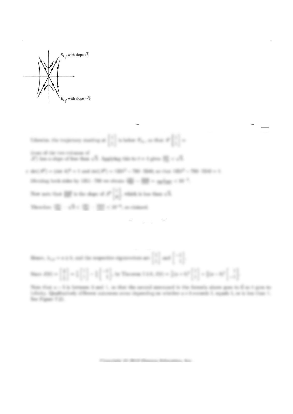
7.4.30 fA(λ) = (2 −λ)2−3 so λ1,2= 2 ±√3 (or approximately 3.73 and 0.27) with eigenvectors 1
√3and −1
√3.
See Figure 7.20.
b The trajectory starting at 0
1is above the line Eλ1, so that At0
1=
343
Chapter 7
Figure 7.20: for Problem 7.4.30a.
(second column of At) has a slope of more than √3, for all t. Applying this to t= 6 gives the estimate √3<1351
780 .
d The slope of A61
1=2131
3691 is less than √3, i.e. 3691
2131 <√3.
7.4.31 The matrix of the dynamical system is A=a b
b a so fA(λ) = (a−λ)2−b2.
7.4.32 C(t+ 1) = 0.8C(t) + 10 so if AC(t)
1=C(t+ 1)
1, A =0.8 10
0 1 .Ahas eigenvectors 1
0,50
1
corresponding to λ1= 0.8 and λ2= 1. Since C(0)
1=0
1, and 0
1=−50 1
0+50
1, we have C(t) =
−50(0.9)t+ 50, hence in the long run, there will be 50 spectators. The graph of C(t) looks similar to the graph
in Figure 7.22.
344
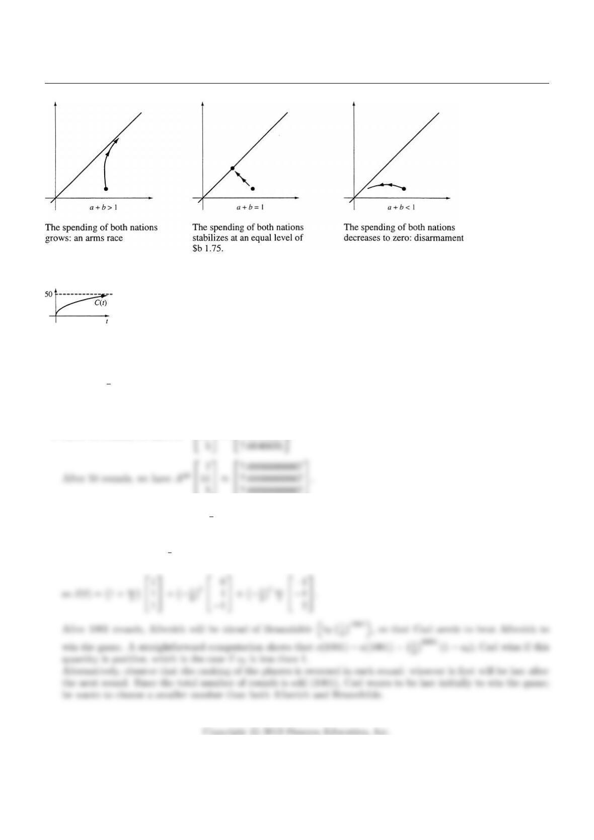
Section 7.4
Figure 7.21: for Problem 7.4.31.
Figure 7.22: for Problem 7.4.32.
7.4.33 aA=1
2
0 1 1
1 0 1
1 1 0
b After 10 rounds, we have A10
7
11
≈
7.6660156
7.6699219
.
c The eigenvalues of Aare 1 and −1
2with
E1= span
1
1
1
and E−1
2= span
0
1
−1
,
−1
−1
2
345
Chapter 7
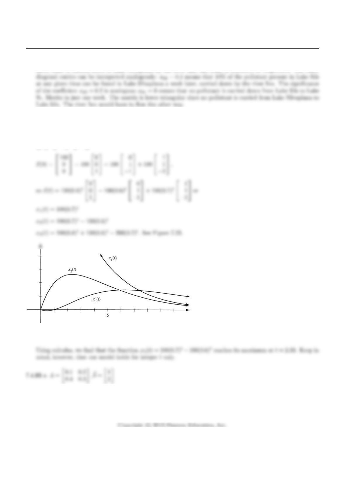
7.4.34 aa11 = 0.7 means that only 70% of the pollutant present in Lake Sils at a given time is still there a week
later; some is carried down to Lake Silvaplana by the river Inn, and some is absorbed or evaporates. The other
b The eigenvalues of Aare 0.8, 0.6, 0.7, with corresponding eigenvectors
0
0
1
,
0
1
−1
,
1
1
−2
.
Figure 7.23: for Problem 7.4.34b.
bB=A~
b
0 1
346
Section 7.4
c The eigenvalues of Aare 0.5 and −0.1 with associated eigenvectors 1
2and 1
−1.
d Write ~y(0) =
x1(0)
x2(0)
1
=c1
1
2
0
+c2
1
−1
0
+c3
2
4
1
.
7.4.36 aT1(t+ 1) = 0.6T1(t) + 0.1T2(t) + 20
T2(t+ 1) = 0.1T1(t) + 0.6T2(t) + 0.1T3(t) + 20
T3(t+ 1) = 0.1T2(t) + 0.6T3(t) + 40
d The eigenvalues of Aare λ1≈0.45858, λ2= 0.6, λ3≈0.74142 so the eigenvalues of Bare λ1≈0.45858, λ2= 0.6,
λ3≈0.74142, λ4= 1.
347
Chapter 7
If ~v1,~v2,~v3are eigenvectors of A(with A~vi=λi~vi), then ~v1
7.4.37 a If ~x(t) =
r(t)
p(t)
w(t)
, then ~x(t+ 1) = A~x(t) with A=
1
2
1
40
1
2
1
2
1
2
01
4
1
2
.
7.4.38 a We are told that
a(t+ 1) = a(t) + j(t)
j(t+ 1) = a(t), so that A=1 1
1 0 .
7.4.39 The eigenfunctions with eigenvalue λare the nonzero functions f(x) such that T(f(x)) = f′(x)−f(x) =
λf(x), or f′(x) = (λ+ 1)f(x). From calculus we recall that those are the exponential functions of the form
f(x) = Ce(λ+1)x, where Cis a nonzero constant. Thus all real numbers are eigenvalues of T, and the eigenspace
Eλis one-dimensional, spanned by e(λ+1)x.
5f(x). From calculus we recall that those are the exponential functions of the form
348
Section 7.4
7.4.42 The nonzero symmetric matrices are eigenmatrices with eigenvalue 0, since L(A) = A−AT=A−A= 0 in
this case. The nonzero skew-symmetric matrices have eigenvalue 2, since L(A) = A−AT=A+A= 2A. Yes, L
is diagonalizable, since we have the eigenbasis 1 0
0 0 ,0 1
1 0 ,0 0
0 1 ,0 1
−1 0 (three symmetric matrices,
and one skew-symmetric one).
7.4.44 The nonzero sequence (x0, x1, x2,…) is an eigensequence with eigenvalue λif
T(x0, x1, x2,…) = (x2, x3, x4,…) = λ(x0, x1, x2,…) = (λx0, λx1, λx2,…). This means that x2=λx0, x3=
7.4.45 The nonzero sequence (x0, x1, x2,…) is an eigensequence with eigenvalue λif
T(x0, x1, x2,…) = (0, x0, x1, x2, . . .) = λ(x0, x1, x2,…) = (λx0, λx1, λx2,…). This means that 0 = λx0, x0=
7.4.46 The nonzero sequence (x0, x1, x2,…) is an eigensequence with eigenvalue λif
T(x0, x1, x2,…) = (x0, x2, x4,…) = λ(x0, x1, x2,…) = (λx0, λx1, λx2,…). This means that x0=λx0, x2=
λx1, x4=λx2,…,x2n=λxn, . . . . For each λ, there are lots of eigensequences: we can choose the terms xk
7.4.47 The nonzero even functions, of the form f(x) = a+cx2, are eigenfunctions with eigenvalue 1, and the nonzero
odd functions, of the form f(x) = bx, have eigenvalue −1. Yes, Tis diagonalizable, since the standard basis,
1, x, x2, is an eigenbasis for T.
7.4.48 Apply Tto the standard basis: T(1) = 1, T (x) = 2x, and T(x2) = (2x)2= 4x2. This gives the eigenvalues