Chapter 7 Rate or direction at any point is changing over time.

7-1

CHAPTER 7

Groundwater – Fundamentals and

One-Dimensional Flow

SOLUTIONS TO QUESTIONS AND PRACTICE PROBLEMS

Section 7.1 Hydrology

7.1 How does groundwater get into the ground?

Solution

Groundwater gets into the ground via infiltration of surface water. The surface water

7.2 Explain the difference between an aquifer, an aquiclude, and an aquitard.

Solution

7.3 Explain the difference between confined flow and unconfined groundwater flow.

Solution

Confined flow, which occurs in a confined aquifer, is that in which both the upper and

Section 7.2 Principles of Fluid Mechanics

7.4 Explain the difference between steady state and unsteady state (transient) flow.

Solution

Steady-state flow means a system has reached equilibrium and the flow rate and direction

7-2 Groundwater – Fundamentals and One-Dimensional Flow Chap. 7

7.5 In most fluid flow application the total head is the sum of the elevation head, pressure

head and velocity head. In groundwater flow we generally assume the velocity is zero.

Why is this a safe assumption?

Solution

In soils, flow rate are very low and the velocity head is much less than either the pressure

7.6 The water in a soil flows from Point K to Point L, a distance of 250 ft. Point K is at

elevation 543 ft and Point L is at elevation 461 ft. Piezometers have been installed at

both points, and their water levels are 23 ft and 74 ft, respectively, above the points.

Compute the average hydraulic gradient between these two points.

Solution

7.7 Compute the pore water pressures at Points K and L in Problem 7.6.

Solution

At Point K:

7.8 The groundwater table in an unconfined aquifer is at a depth of 9.3 m below the ground

surface. Assuming hydrostatic conditions are present, and the groundwater is virtually

stationary, compute the pore water pressure at depths of 15.0 and 20.0 m below the

ground surface.

Solution

At 15.0 m:

Chap. 7 Groundwater – Fundamentals and One-Dimensional Flow 7-3

7.9 An exploratory boring is being drilled. The soil encountered between the ground surface

and a depth of 10 m has been dry sand, with no visible signs of groundwater. Then, at a

depth of 10 m the soil changes to a moist clay which becomes very wet at a depth of 12 m.

At 12 m the soil changes back to a silty sand which is very wet. The boring continues to a

depth of 15 m. A piezometer is then installed in the lower silty sand layer. Within 2 days,

the water in the piezometer had risen to a depth of only 8 m below the ground surface.

Explain the groundwater conditions that have been encountered.

Solution

The silty sand encountered at a depth of 12m is an a confined aquifer in an artesian

7.10 Compute the pore water pressures at the bottom of the piezometer in Problem 7.9.

Solution

7.11 Two small commercial buildings have been constructed at a site underlain by a sandy silt

(ML) that has D10 = 0.03 mm. The groundwater table is at a depth of 6 ft. Both buildings

have concrete slab-on-grade floors. In Building A, the slab was placed directly onto the

natural soils, while Building B has a 4-inch layer of poorly- graded coarse gravel between

the slab and the natural soils. Both buildings have vinyl floor coverings similar to those

typically used in residential kitchens. Both buildings are now three years old.

Unfortunately, the tenant in Building A is having continual problems with the

vinyl floors peeling up from the concrete slab. When the peeled sections are examined,

moisture is always evident between the vinyl and the concrete. Curiously, the tenant in

Building B has had no such problems, even though both buildings have the same floor

covering. Could the problem in Building A be due to capillary action in the underlying

soil? Explain why or why not. Also explain why Building B is not having any such

problems.

Solution

The potential height of capillary rise in this soil is approximately

7-4 Groundwater – Fundamentals and One-Dimensional Flow Chap. 7

7.12 A certain clayey zone has a zone of capillary rise of 4.5 m above the groundwater table.

What is the pressure head and the pore pressure at a point 2 m above the groundwater

table?

Solution

By definition the pore pressure and pressure head at the elevation of the

Section 7.3 One-Dimensional Flow Through Soil

7.13 A constant-head hydraulic conductivity test has been conducted on a 110 mm diameter,

270 mm tall fine sand specimen in a permeameter similar to the one shown in Figure 7.18.

The upper and lower reservoir elevations were 2010 mm and 1671 mm above the lab

floor. The piezometers, whose tips are spaced 200 mm apart, had readings of 1809 and

1578 mm, and the graduated cylinder collected 910 ml of water in 25 min 15 s. Using the

best available data, compute the hydraulic conductivity. Does the result seem

reasonable? Why or why not?

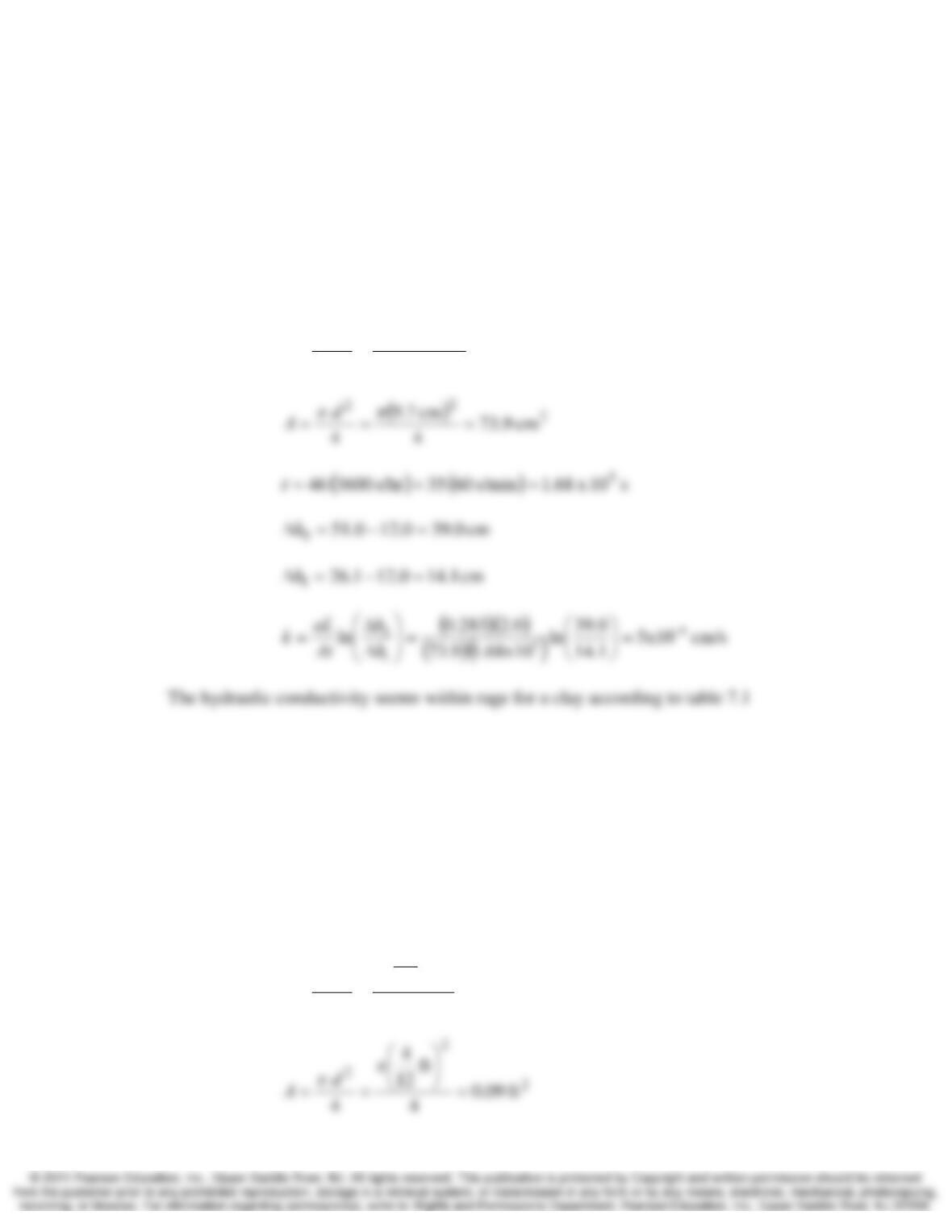
Solution

The piezometers provide more accurate measurements of i, than do the elevations of the

two reservoirs. Therefore computations using the piezometer measurements are preferred.

Chap. 7 Groundwater – Fundamentals and One-Dimensional Flow 7-5

7.14 A falling-head hydraulic conductivity test has been conducted on a clay specimen in a

permeameter similar to the one in Figure 7.19. The soil specimen was 97 mm in diameter

and 20 mm tall. The standpipe had an inside diameter of 6.0 mm. The water level in the

bath surrounding the specimen was 120 mm above the laboratory counter top and the

water level in the standpipe fell from a height of 510 mm to 261 mm above the counter

top in 46 hours 35 minutes. Compute the hydraulic conductivity. Does the result seem

reasonable? Why or why not?

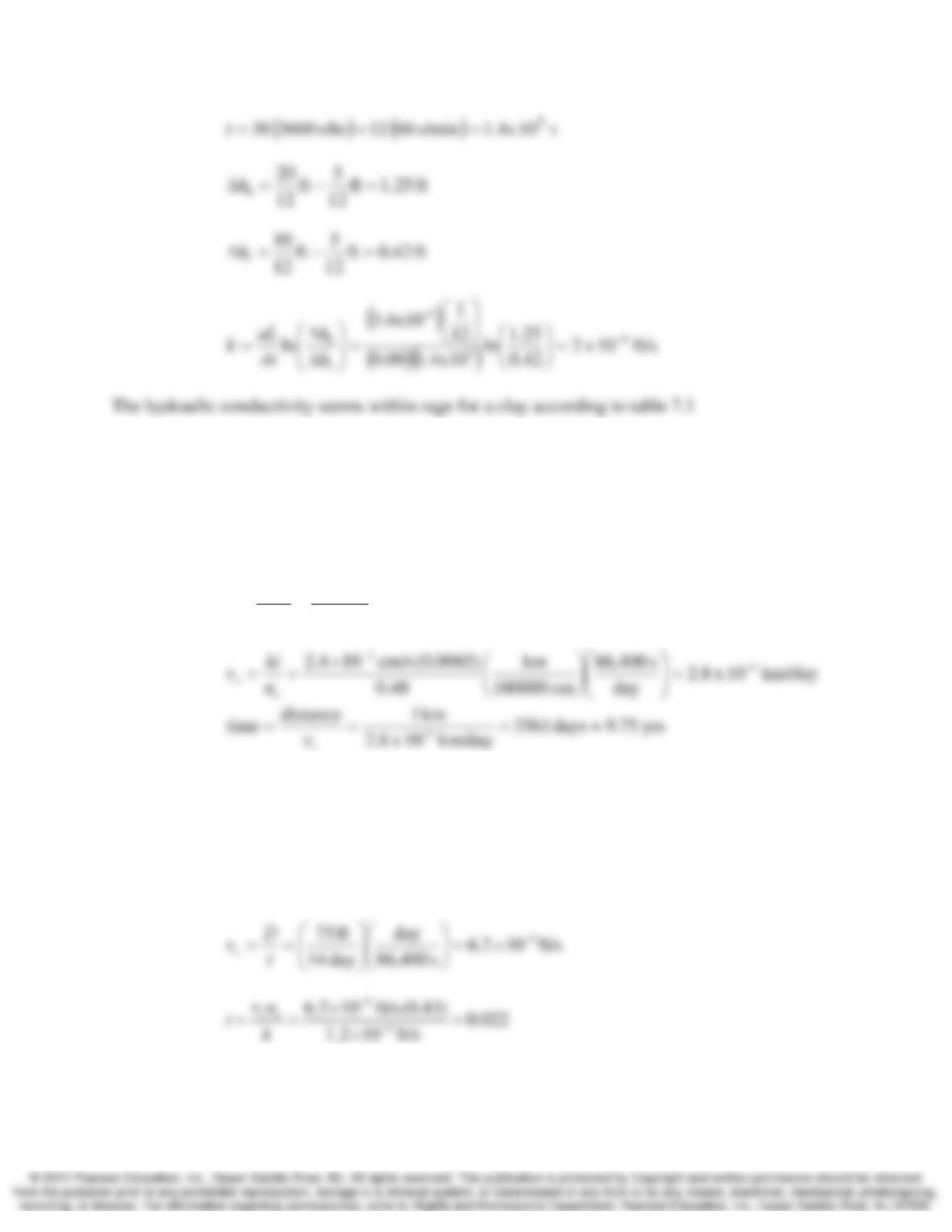
Solution

(

)

2

cm 283.0

4

cm 0.60

4

=== πd

a

π

7.15 A falling-head hydraulic conductivity test has been conducted on a clay specimen in a

permeameter similar to the one in Figure 7.19. The soil specimen was 4 in. in diameter

and 1 in. tall. The standpipe had an inside diameter of 0.25 in. The water level in the bath

surrounding the specimen was 5 in. above the laboratory counter top and the water level

in the standpipe fill from a height of 20 in. to 10 in. above the counter top in 38 hours 12

minutes. Compute the hydraulic conductivity in ft/s. Does the result seem reasonable?

Why or why not?

Solution

24

2

ft 104.3

4

ft

12

.25

4

−

=

⎟

⎠

⎞

⎜

⎝

⎛

== x

π

d

a

π

7-6 Groundwater – Fundamentals and One-Dimensional Flow Chap. 7

7.16 A certain 20 m thick sandy confined aquifer has a hydraulic conductivity of 2.4 x 10-2

cm/s and a void ratio of 0.91. Groundwater is flowing through this aquifer with a

hydraulic gradient of 0.0065. How much time would be required for water to travel 1 km

through this aquifer?

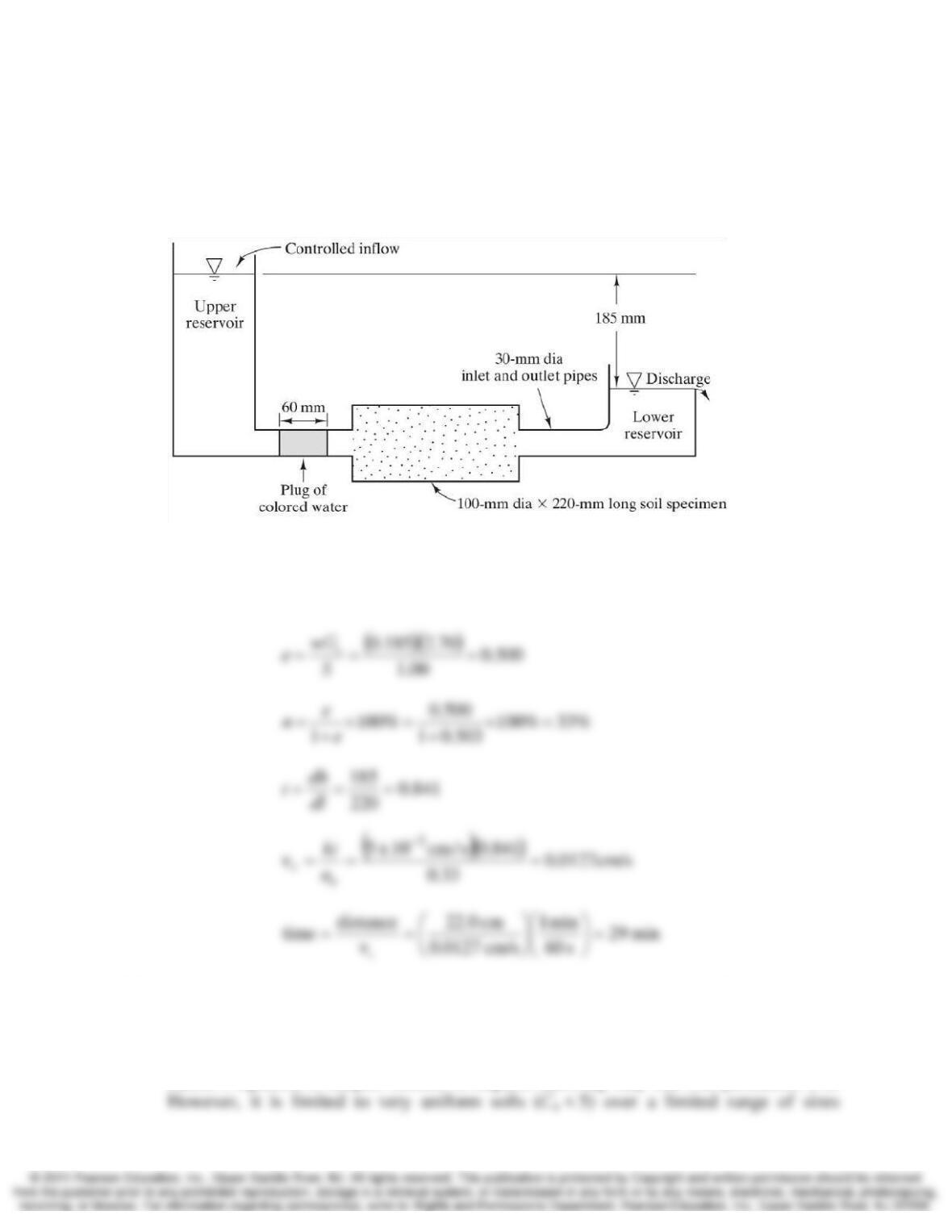
Solution

%48

91.01

91.0

1=

+

=

+

=e

e

n

7.17 A tracer dye is injected into a 55 foot thick sandy gravel confined aquifer which has a

hydraulic conductivity of 1.2 x 10-3 ft/s. The dye appears 14 days later in an observation

well 75 feet away from the injection point. Compute the seepage velocity and estimate

the hydraulic gradient in the aquifer if the porosity of the soil is 42%?

Solution

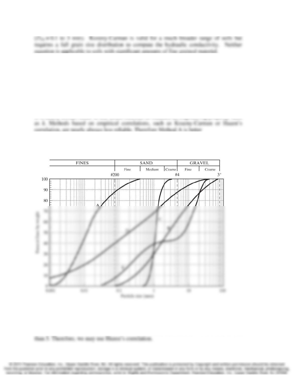
7.18 The laboratory apparatus shown in Figure 7.22 maintains a constant head in both the

upper and lower reservoirs. The soil sample is a silty sand (SM) with k = 5×10-3 cm/s

Chap. 7 Groundwater – Fundamentals and One-Dimensional Flow 7-7

and w = 18.5%. Assume a reasonable value for Gs, then determine the time required for

the plug of colored water to pass through the soil or absorption (i.e., from when the

leading edge first enters the soil to when it begins to exit). Assume the colored water

travels only through advection and it has the same unit weight and viscosity as plain

water.

Figure 7.22 Laboratory apparatus for Problem 7.18.

Solution

Assume Gs=2.70 (from suggested values in Chapter 4, pg 128)

7.19 What are the pros and cons of using Hazen’s equation versus the Kozeny-Carman

equation for estimating hydraulic conductivity of a coarse grained soil?

Solution

Hazen’s equation is simpler because it requires knowing only one soil parameter, D10.

7-8 Groundwater – Fundamentals and One-Dimensional Flow Chap. 7

7.20 Which of the following methods would be the better way to determine k for a clean sand?

Why?

(a) Place a soil sample in a constant-head permeameter, conduct a hydraulic

conductivity test, and compute k using Equation 7.10.

(b) Conduct a sieve analysis and compute k using Equation 7.20.

Solution

It is nearly always better to use direct methods to measure an engineering property, such

correlation, are nearly always less reliable. Therefore Method A is better

7.21 May we use the Hazen correlation to estimate the hydraulic conductivity for soil C in

Figure 4.13? Why or why not? If so, compute k.

Figure 4.13 Particle size distribution curves for five soils (Soil A through Soil E)

Solution

D10=0.75mm, which is between 0.1 and 3.0 mm, and Cu=1.2/0.75 = 1.6, which is less

Chap. 7 Groundwater – Fundamentals and One-Dimensional Flow 7-9

7.22 Compute the hydraulic conductivity for subrounded poorly graded soil C in Figure 4.13

using the Kozeny-Carmen equation (Eq 7.20).

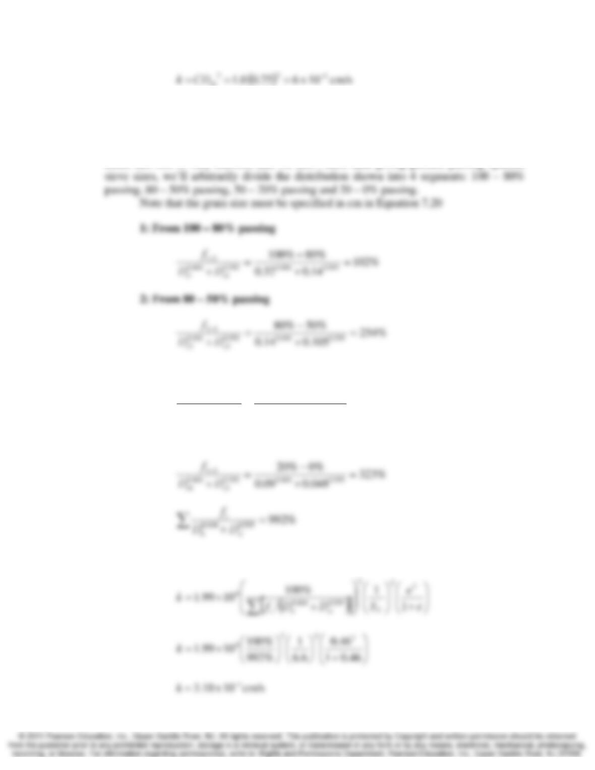
Solution

Since this soil is very uniform and we don’t have data giving percent passing specific

3: From 50 – 20% passing

%313

09.0105.0

%20%50

595.0404.0595.0

3

404.0

3

43 =

×

−

=

×

−

sl DD

f

4: From 20 – 0% passing

For subrounded soil SF = 6.6, Table 7.2

7-10 Groundwater – Fundamentals and One-Dimensional Flow Chap. 7

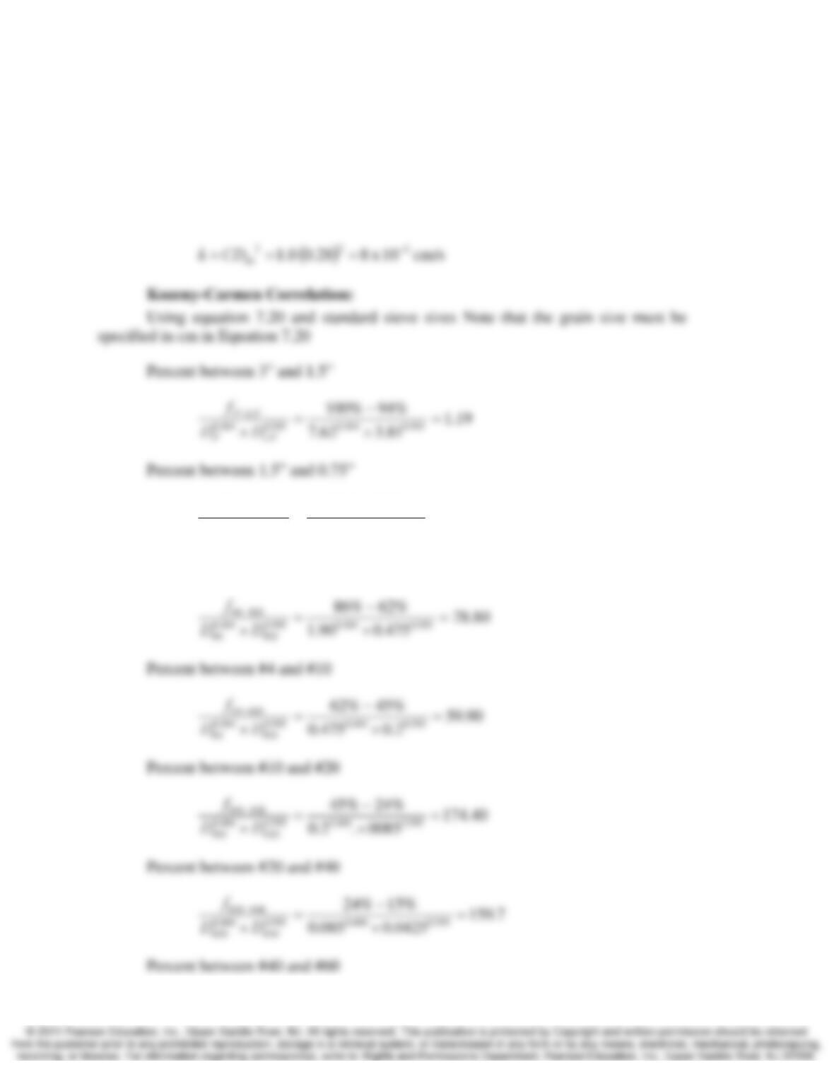
7.23 Compute the hydraulic conductivity for subangular coarse grained soil B in Figure 4.13

using both Hazen’s correlation the Kozeny-Carmen equation (Eq 7.20). Assume a void

ratio of 48%

Solution

Hazen’s correlation:

18.3

90.181.3

%86%94

595.0404.0595.0

“75.0

404.0

“5.1

“75.0“5.1 =

×

−

=

×

−

DD

f

Percent between 0.75” and #4

Chap. 7 Groundwater – Fundamentals and One-Dimensional Flow 7-11

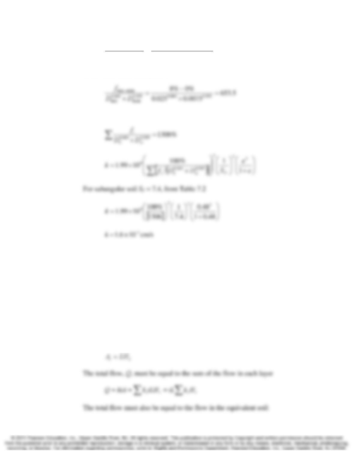
3.225

025.00425.0

%8%15

595.0404.0595.0

60#

404.0

40#

60#40# =

×

−

=

×

−

DD

f

Percent between #60 and #200

Section 7.4 Flow Through Anisotropic Soils

7.24 Derive Equations 7.23 and 7.26.

Solution

Hint: For Equation 7.23, write Darcy’s law for horizontal flow using the real soil

(k=k1, k2, etc), the write it again using the equivalent soil (k=kx). Since Q is the same for

both, you can then solve for kx.

Equation 7.23:

Consider a width L measured perpendicular to the direction of flow. For each

layer, i