133
18. a., b., & c. The regression results follow.
The regression equation is
Predictor Coef SE Coef T P VIF
Constant -43.15 31.67 -1.36 0.192
Analysis of Variance
Source DF SS MS F P
Unusual Observations
New
The variance inflation factors (VIF all small (near 1); however, the t ratios and
134
19. Stepwise regression results, with significance level .05 to enter and leave the
regression function, follow.
Step 1
All possible regression results are summarized in the following table.
Predictor
Variables
2
R
X1
.295
X2
.301
X3
.377
X1, X2
.404
X
1, X3
.452
X2, X3
.460
X
1, X2, X3
.498
The
2
R
criterion would suggest using all three predictor variables. However, the
20. Best three predictor variable model selected by stepwise regression follows.
The regression equation is
135
Coefficient on education is negative. Everything else equal, as education level
Unusual Observations
Observation 31 has a large standardized residual and is influential. Observation 33
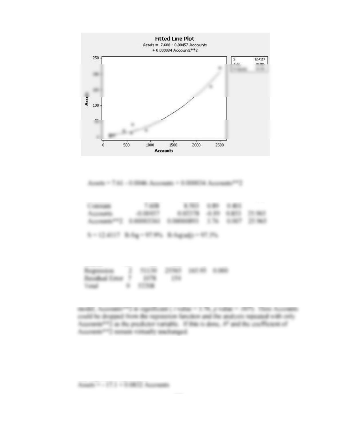
21. Scatter diagram with fitted quadratic regression function:
136
a. & b. The regression equation is
Predictor Coef E Coef T P VIF
Analysis of Variance
Source DF SS MS F P
The regression is significant (F = 165.95, p value = .000). Given Accounts in the
c. Dropping Accounts**2 from the model gives:
The regression equation is
137
Predictor Coef SE Coef T P
22. The final model:
The regression equation is
Predictor Coef SE Coef T P VIF
Analysis of Variance
Source DF SS MS F P
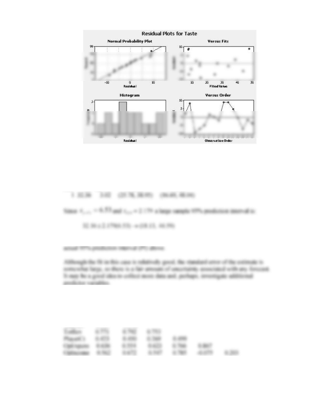
function is adequate. There is no reason to doubt the usual regression assumptions.
138
23. Using the final model from problem 22 with H2S = 7.3 and Lactic = 1.85
Predicted Values for New Observations
New
Obs Fit SE Fit 95% CI 95% PI
Notice the large sample 95% prediction interval is not too much different than the
24. a. Correlations: GtReceit, MediaRev, StadRev, TotRev, PlayerCt, OpExpens, …
GtReceit MediaRev StadRev TotRev PlayerCt OpExpens OpIncome
MediaRev 0.304
StadRev 0.587 0.348
139
b. Stepwise Regression: FranValu versus GtReceit, MediaRev, …
Step 1
Constant 2.928
c. The coefficient of TotRev from the stepwise program is 1.96 and the constant
d. The regression equation is
OpExpens = 18.9 + 1.30 PlayerCt
Source DF SS MS F P
Unusual Observations
Obs PlayerCt OpExpens Fit SE Fit Residual St Resid
140
e. Clearly Total revenue, Operating expenses and Operating income are
CASE 7-1: THE BOND MARKET
The actual data for this case is supplied in Appendix A. Students can either be asked to
1. What questions do you think Judy will have for Ron? The students always seem
to come up with questions that Ms. Johnson will ask. The key is that Ron should be able
to answer them. Possible issues include:
Are all the predictor variables in the final model required? Is a simpler model
with fewer predictor variables feasible?
CASE 7-2: AAA WASHINGTON
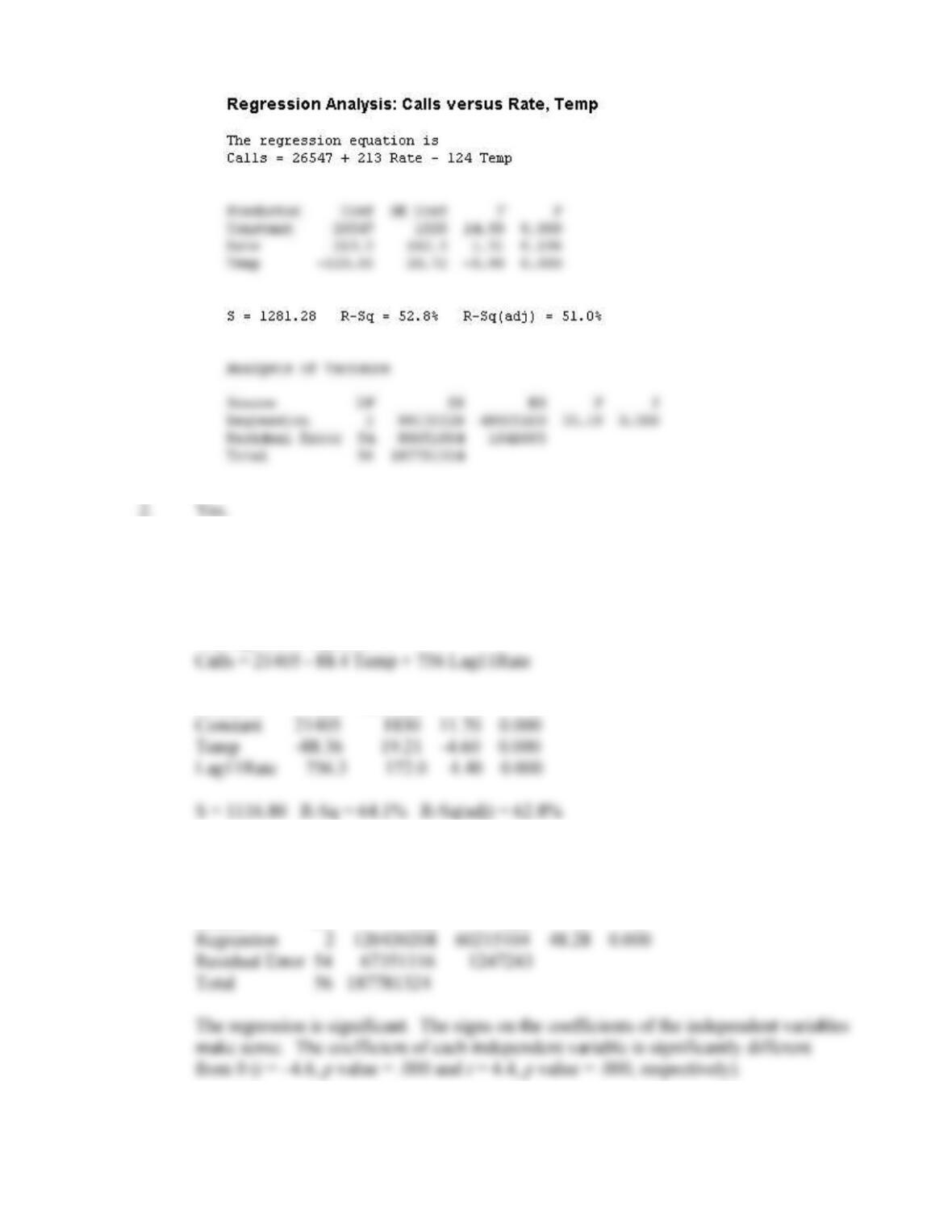
1. The multiple regression model that includes both unemployment rate and average
monthly temperature is shown below. Temperature is the only good predictor variable.
141
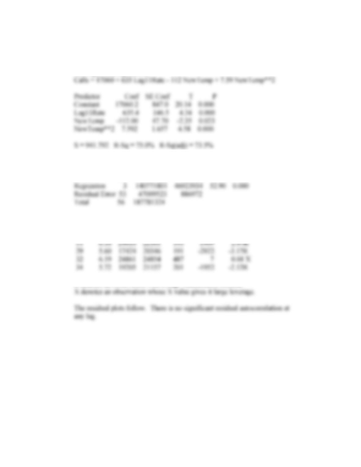
3. Unemployment rate lagged 11 months is a good predictor of emergency road service
calls. Unemployment rate lagged 3 months is not a good predictor. The Minitab output
with Temp and Lagged11Rate is given below.
The regression equation is
Predictor Coef SE Coef T P
Analysis of Variance
Source DF SS MS F P
142
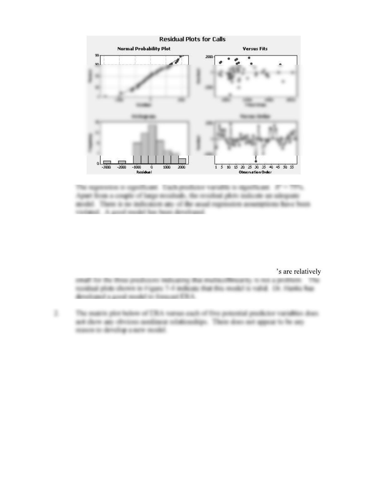
4. The results for a regression model with independent variables unemployment
rate lagged 11 months (Lag11Rate), transformed average temperature (NewTemp)
and NewTemp**2 are given below.
The regression equation is
Analysis of Variance
Source DF SS MS F P
Unusual Observations
Obs Lag11R Calls Fit SE Fit Residual St Resid
R denotes an observation with a large standardized residual.
143
CASE 7-3: FANTASY BASEBALL (A)
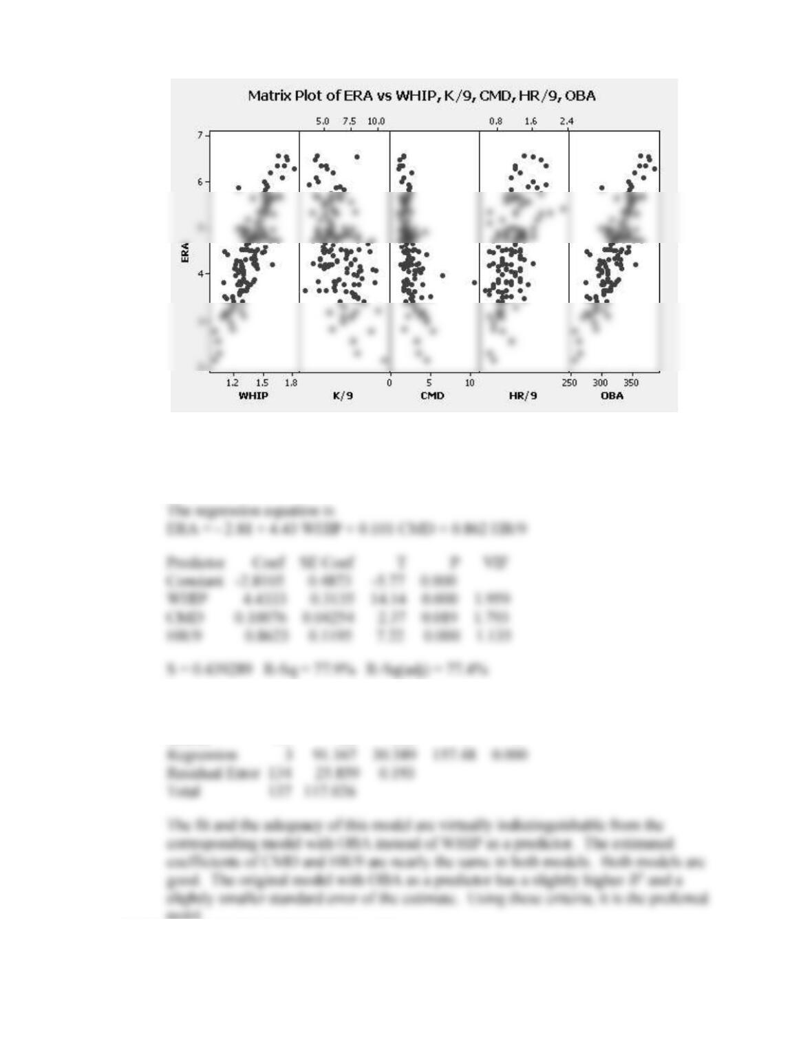
1. The regression is significant. The R
2
of 78.1% looks good. The t statistic for each
of the predictor variables is large with a very small p-value. The VIF
144
3. The regression results with WHIP replacing OBA as a predictor variable follow.
The residual plots are very similar to those in Figure 7-4.
Analysis of Variance
Source DF SS MS F P
model.
CASE 7-4: FANTASY BASEBALL (B)
145
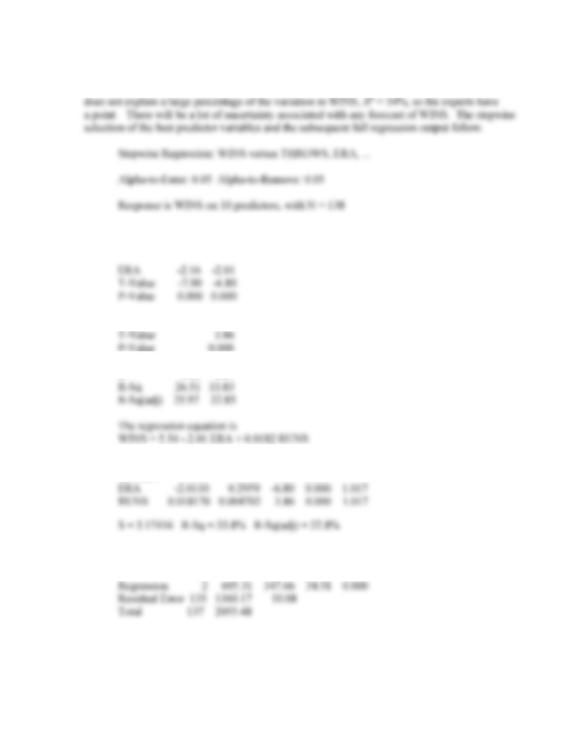
The project may not be doomed to failure. A lot can be learned from investigating the
influence of the various independent variables on WINS. However, the best regression model
Step 1 2
Constant 20.531 5.543
RUNS 0.0182
S 3.33 3.17
Predictor Coef SE Coef T P VIF
Constant 5.543 4.108 1.35 0.179
Analysis of Variance
Source DF SS MS F P