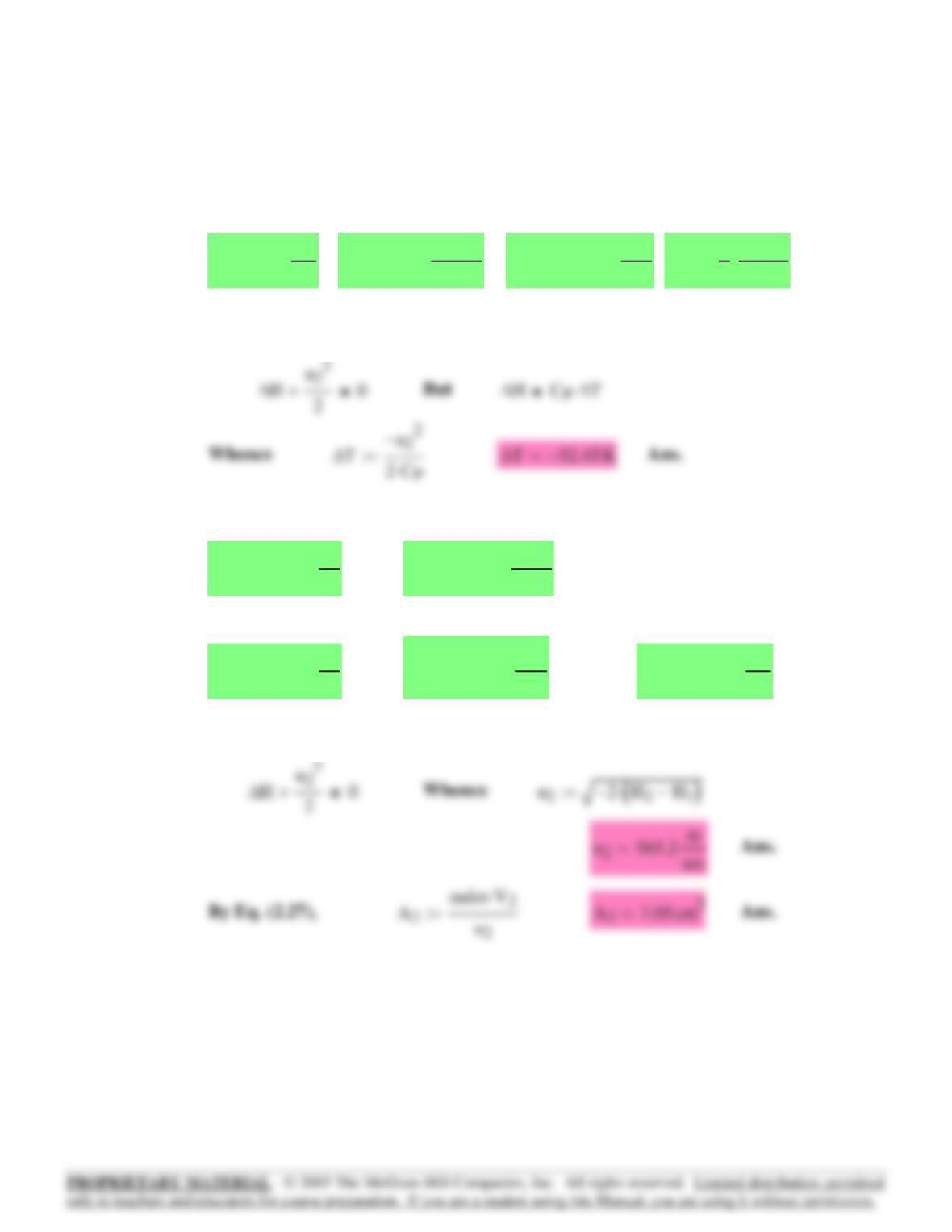
Interpolation in Table F.2 at P = 525 kPa and S = 7.1595 kJ/(kg*K) yields:
H22855.2 kJ
kg
⋅:= V2531.21 cm3
gm
⋅:= mdot 0.75 kg
sec
⋅:=
With the heat, work, and potential-energy terms set equal to zero and
with the initial velocity equal to zero, Eq. (2.32a) reduces to:
7.5 The calculations of the preceding problem may be carried out for a
series of exit pressures until a minimum cross-sectional area is found.
The corresponding pressure is the minimum obtainable in the converging
nozzle. Initial property values are as in the preceding problem.
Chapter 7 – Section A – Mathcad Solutions
7.1 u2325 m
sec
⋅:= R 8.314 J
mol K⋅
⋅:= molwt 28.9 gm
mol
:= CP
7
2
R
molwt
⋅:=
With the heat, work, and potential-energy terms set equal to zero and
with the initial velocity equal to zero, Eq. (2.32a) reduces to
7.4 From Table F.2 at 800 kPa and 280 degC:
H13014.9 kJ
kg
⋅:= S17.1595 kJ
kg K⋅
⋅:=
220

(guess)
pmin 400 kPa⋅:=
AP( ) interp s p,a2
,P,
()
:=s cspline P A2
,
()
:=
a2iA2i
:=piPi
:=i15..:=
Fit the P vs. A2 data with cubic spline and find
the minimum P at the point where the first
derivative of the spline is zero.
7.05
7.022
⎛
⎜
⎞
565.2
541.7
⎛
⎜
⎞
A2
mdot V2
⋅
u2
→
⎯
⎯
⎯
:=u22−H2H1
−
()
⋅
→
⎯
⎯⎯⎯⎯
⎯
:=mdot 0.75 kg
sec
⋅:=
V2
531.21
507.12
485.45
465.69
447.72
⎛
⎜
⎜
⎜
⎜
⎜
⎝
⎞
⎟
⎟
⎟
⎠
cm3
gm
⋅:=H2
2855.2
2868.2
2880.7
2892.5
2903.9
⎛
⎜
⎜
⎜
⎜
⎜
⎝
⎞
⎟
⎟
⎟
⎠
kJ
kg
⋅:=P
400
425
450
475
500
⎛
⎜
⎜
⎜
⎜
⎜
⎝
⎞
⎟
⎟
⎟
⎠
kPa⋅:=
Interpolations in Table F.2 at several pressures and at the given
entropy yield the following values:
S2S1
=S17.1595 kJ
kg K⋅
⋅:=H13014.9 kJ
kg
⋅:=
221
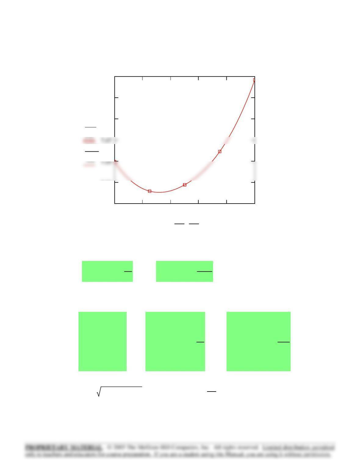
Show spline fit graphically: p 400 kPa⋅401 kPa⋅, 500 kPa⋅..:=
400 420 440 460 480 500
7.01
7.03
7.09
7.11
7.13
A2i
Ap()
Pi
kPa
p
kPa
,
7.9 From Table F.2 at 1400 kPa and 325 degC:
H13096.5 kJ
kg
⋅:= S17.0499 kJ
kg K⋅
⋅:= S2S1
:=
Interpolate in Table F.2 at a series of downstream pressures and at S =
7.0499 kJ/(kg*K) to find the minimum cross-sectional area.
P
800
775
750
725
700
⎛
⎜
⎜
⎜
⎜
⎜
⎝
⎞
⎟
⎟
⎟
⎠
kPa⋅:= H2
2956.0
2948.5
2940.8
2932.8
2924.9
⎛
⎜
⎜
⎜
⎜
⎜
⎝
⎞
⎟
⎟
⎟
⎠
kJ
kg
⋅:= V2
294.81
302.12
309.82
317.97
326.69
⎛
⎜
⎜
⎜
⎜
⎜
⎝
⎞
⎟
⎟
⎟
⎠
cm3
gm
⋅:=
u22−H2H1
−
()
⋅
→
⎯
⎯⎯⎯⎯
⎯
:= A2
V2
u2
⎛
⎜
⎝
⎞
⎠mdot⋅=
222

Svap 1.6872 Btu
lbmrankine⋅
⋅:=Sliq 0.3809 Btu
lbmrankine⋅
⋅:=
Hvap 1167.1 Btu
lbm
⋅:=Hliq 228.03 Btu
lbm
⋅:=
From Table F.4 at 35(psi), we see that the final state is wet steam:
H21154.8 Btu
lbm
=H2H1∆H+:=
∆H 78.8−Btu
lbm
=∆Hu12u22
−
2
:=
By Eq. (2.32a),
S11.6310 Btu
lbmrankine⋅
⋅:=H11233.6 Btu
lbm
⋅:=
From Table F.4 at 130(psi) and 420 degF:
u22000 ft
sec
⋅:=u1230 ft
sec
⋅:=
7.10
At the nozzle exit, P = 140 kPa and S = S1, the initial value. From
Table F.2 we see that steam at these conditions is wet. By
V2
u2
⎛
⎜
⎝
⎞
⎠
→
⎯
⎯
5.561
5.553
5.552
5.557
⎛
⎜
⎜
⎜
⎜
⎜
⎞
⎟
⎟
⎟
cm2sec⋅
kg
=
Since mdot is constant,
the quotient V2/u2 is a
measure of the area. Its
minimum value occurs very
close to the value at
vector index i = 3.
223

7.12 Values from the steam tables for saturated-liquid water:
At 15 degC: V 1.001 cm3
gm
⋅:= T 288.15 K⋅:=
Enthalpy difference for saturated liquid for a temperature change from
14 to 15 degC:
∆H 67.13 58.75−()
J
gm
⋅:= ∆t2K⋅:= Cp ∆H
∆t
:=
Cp 4.19 J
gm K⋅
=
β1.5 10 4−
⋅
K
:= ∆P4−atm⋅:=
Apply Eq. (7.25) to the constant-enthalpy throttling process. Assumes
very small temperature change and property values independent of P.
xH2Hliq
−
Hvap Hliq
−
:= x 0.987=(quality)
7.11 u2580 m
sec
⋅:= T2273.15 15+()K⋅:= molwt 28.9 gm
mol
:= CP
7
2
R
molwt
⋅:=
By Eq. (2.32a), ∆Hu12u22
−
2
=
u22
−
2
=
224

D
1.157−
0.0
0.040
0.0
⎛
⎜
⎜
⎜
⎜
⎝
⎞
⎟
⎟
⎠
105
⋅K2
⋅:=
C
0.0
4.392−
0.0
8.824−
⎛
⎜
⎜
⎜
⎜
⎝
⎞
⎟
⎟
⎠
10 6−
K2
⋅:=
B
1.045
14.394
.593
28.785
⎛
⎜
⎜
⎜
⎜
⎝
⎞
⎟
⎟
⎠
10 3−
K
⋅:=A
5.457
1.424
3.280
1.213
⎛
⎜
⎜
⎜
⎜
⎝
⎞
⎟
⎟
⎠
:=
ω
.224
.087
.038
.152
⎛
⎜
⎜
⎜
⎜
⎝
⎞
⎟
⎟
⎠
:=
Pc
73.83
50.40
34.00
42.48
⎛
⎜
⎜
⎜
⎜
⎝
⎞
⎟
⎟
⎠
bar:=
Tc
304.2
282.3
126.2
369.8
⎛
⎜
⎜
⎜
⎜
⎝
⎞
⎟
⎟
⎠
K:=
P1
80
60
60
20
⎛
⎜
⎜
⎜
⎜
⎝
⎞
⎟
⎟
⎠
bar:=
T1
350
350
250
400
⎛
⎜
⎜
⎜
⎜
⎝
⎞
⎟
⎟
⎠
K:=
P2 1.2bar:=
7.13–7.15
∆S 1.408 10 3−
×J
gm K⋅
=∆SCpln
T∆T+
T
⎛
⎜
⎝
⎞
⎠
⋅βV⋅∆P⋅−:=
The entropy change for this process is given by Eq. (7.26):
∆T 0.093 K=∆TV−1βT⋅−
()
⋅∆P⋅
Cp
1
9.86923
joule
cm3atm⋅
⋅
⎛
⎜
⎝
⎞
⎠
⋅:=
225

T2
280
302
232
385
⎛
⎜
⎜
⎜
⎜
⎝
⎞
⎟
⎟
⎠
K:=
Guesses
The simplest procedure here is to iterate by guessing T2, and then
calculating it.
Eq. (6.65b)
Iiln Zβiqi
,
()
βi
+
Zβiqi
,
()
⎛
⎜
⎝
⎞
⎠
:=
i14..:=
Zβq,
()
Find z():=
Eq. (3.52)
z1β+ qβ⋅ zβ−
zz β+
()
⋅
⋅−=
As in Example 7.4, Eq. (6.93) is applied to this constant-enthalpy
process. If the final state at 1.2 bar is assumed an ideal gas, then Eq.
(A) of Example 7.4 (pg. 265) applies. Its use requires expressions for HR
and Cp at the initial conditions.
Tr T1
Tc
→
⎯
:= Tr
1.151
1.24
1.981
1.082
⎛
⎜
⎜
⎜
⎜
⎝
⎞
⎟
⎟
⎠
=Pr P1
Pc
→
⎯
:= Pr
1.084
1.19
1.765
0.471
⎛
⎜
⎜
⎜
⎜
⎝
⎞
⎟
⎟
⎠
=
7.13 Redlich/Kwong equation: Ω0.08664:= Ψ 0.42748:=
βΩ
Pr
Tr
⋅
⎛
⎜
⎝
⎞
⎠
→
⎯
⎯
⎯
:= Eq. (3.53) qΨ
ΩTr1.5
⋅
⎛
⎜
⎝
⎞
⎠
→
⎯
⎯⎯
⎯
:= Eq. (3.54)
Guess: z1:=
Given
226

α1c1Tr
0.5
−
()
⋅+
⎡
⎣
⎤
⎦
2
→
⎯
⎯⎯⎯⎯⎯⎯
⎯
:=
βΩ
Pr
Tr
⋅
⎛
⎜
⎝
⎞
⎠
→
⎯
⎯
⎯
:= Eq. (3.53) qΨα⋅
ΩTr⋅
⎛
⎜
⎝
⎞
⎠
→
⎯
⎯
⎯
:= Eq. (3.54)
Guess: z1:=
Given z1β+ qβ⋅ zβ−
zz β+
()
⋅
⋅−=Eq. (3.52) Zβq,
()
Find z():=
i14..:= Iiln Zβiqi
,
()
βi
+
Zβiqi
,
()
⎛
⎜
⎝
⎞
⎠
:= Eq. (6.65b)
Zβiqi
,
()
0.721
0.773
0.956
0.862
=
HR
2.681−
2.253−
0.521−
1.396−
⎛
⎜
⎜
⎜
⎜
⎝
⎞
⎟
⎟
⎠
kJ
mol
=SR
5.177−
4.346−
1.59−
2.33−
⎛
⎜
⎜
⎜
⎜
⎝
⎞
⎟
⎟
⎠
J
mol K⋅
=
τT2
T1
→
⎯
:= Cp R A B
2T1⋅τ1+
()
⋅+ C
3T12
⋅τ
2τ+ 1+
()
⋅+ D
τT12
⋅
+
⎡
⎢
⎣
⎤
⎥
⎦
⋅
⎡
⎢
⎣
⎤
⎥
⎦
→
⎯
⎯⎯⎯⎯⎯⎯⎯⎯⎯⎯⎯⎯⎯⎯⎯⎯⎯⎯⎯⎯⎯
⎯
:=
T2 HR
Cp T1+
⎛
⎜
⎝
⎞
⎠
→
⎯
⎯⎯
⎯
:= ∆SCpln
T2
T1
⎛
⎜
⎝
⎞
⎠
⋅Rln P2
P1
⎛
⎜
⎝
⎞
⎠
⋅− SR−
⎛
⎜
⎝
⎞
⎠
→
⎯
⎯⎯⎯⎯⎯⎯⎯⎯⎯⎯⎯
⎯
:=
⎜
⎜
⎜
⎜
7.14 Soave/Redlich/Kwong equation: Ω0.08664:= Ψ 0.42748:=
c 0.480 1.574 ω⋅+ 0.176 ω2
⋅−
()
→
⎯
⎯⎯⎯⎯⎯⎯⎯⎯⎯⎯
⎯
:=
227
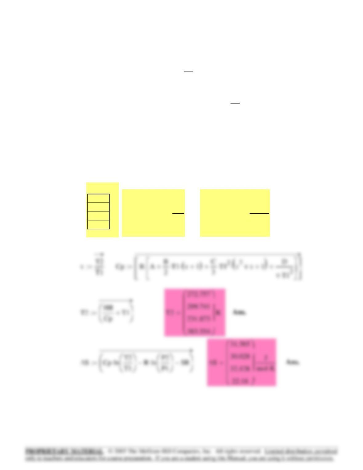
SR
6.126−
4.769−
1.789−
2.679−
⎛
⎜
⎜
⎜
⎜
⎝
⎞
⎟
⎟
⎠
J
mol K⋅
=HR
2.936−
2.356−
0.526−
1.523−
⎛
⎜
⎜
⎜
⎜
⎝
⎞
⎟
⎟
⎠
kJ
mol
=
Zβiqi
,
()
0.75
0.79
0.975
0.866
=
T2
273
300
232
384
⎛
⎜
⎜
⎜
⎜
⎝
⎞
⎟
⎟
⎠
K:=
Guesses
Now iterate for T2:
ci
−Tri
αi
⎛
⎜
⎝
⎞
⎠
0.5
⋅
The derivative in these equations equals:
Eq. (6.68)
SRiRlnZβiqi
,
()()
βi
−ci
Tri
αi
⎛
⎜
⎝
⎞
⎠
0.5
⋅qi
⋅Ii
⋅−
⎡
⎢
⎣
⎤
⎥
⎦
⋅:=
228
⎜
⎜
⎜
⎜
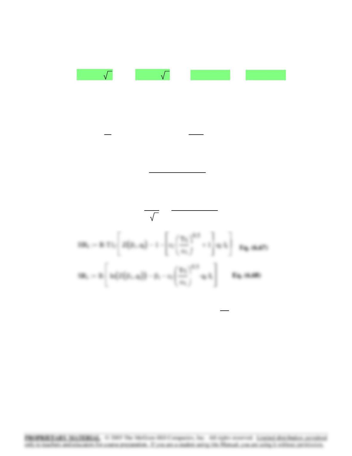
T2
270
297
229
383
⎛
⎜
⎜
⎜
⎜
⎝
⎞
⎟
⎟
⎠
K:=
Guesses
Now iterate for T2:
ci
−Tri
αi
⎛
⎜
⎝
⎞
⎠
0.5
⋅
The derivative in these equations equals:
Eq. (6.65b)
Ii
1
22
⋅ln Zβiqi
,
()
σβ
i
⋅+
Zβiqi
,
()
εβ
i
⋅+
⎛
⎜
⎝
⎞
⎠
⋅:=
i14..:=
Zβq,
()
Find z():=
Eq. (3.52)
z1β+ qβ⋅ zβ−
zεβ⋅+
()
zσβ⋅+
()
⋅
⋅−=Given
z1:=
Guess:
Eq. (3.54)
qΨα⋅
ΩTr⋅
⎛
⎜
⎝
⎞
⎠
→
⎯
⎯
⎯
:=
Eq. (3.53)
βΩ
Pr
Tr
⋅
⎛
⎜
⎝
⎞
⎠
→
⎯
⎯
⎯
:=
α1c1Tr
0.5
−
()
⋅+
⎡
⎣
⎤
⎦
2
→
⎯
⎯⎯⎯⎯⎯⎯
⎯
:=c 0.37464 1.54226 ω⋅+ 0.26992 ω2
⋅−
()
→
⎯
⎯⎯⎯⎯⎯⎯⎯⎯⎯⎯⎯⎯⎯
⎯
:=
Ψ0.45724:=Ω 0.07779:=ε 12−:=σ 12+:=
Peng/Robinson equation:7.15
229
⎜
⎜
(quality)
x 0.92=xS2Sliq
−
Svap Sliq
−
:=
S2S1
:=Svap 7.9094 kJ
kg K⋅
⋅:=Sliq 0.8321 kJ
kg K⋅
⋅:=
For isentropic expansion, exhaust is wet steam:
By Eq. (7.13),
S17.3439 kJ
kg K⋅
⋅:=H22609.9 kJ
kg
⋅:=H13462.9 kJ
kg
⋅:=
Data from Table F.2:
Wdot 3500−kW⋅:=
7.18
⎜
⎜
⎜
⎜
SR
6.152−
4.784−
1.847−
2.689−
⎛
⎜
⎜
⎜
⎜
⎝
⎞
⎟
⎟
⎠
J
mol K⋅
=HR
3.041−
2.459−
0.6−
1.581−
⎛
⎜
⎜
⎜
⎜
⎝
⎞
⎟
⎟
⎠
kJ
mol
=
Zβiqi
,
()
0.722
0.76
0.95
0.85
=
230
7.19 The following vectors contain values for Parts (a) through (g). For intake
conditions:
H1
3274.3 kJ
kg
⋅
3509.8 kJ
kg
⋅
⎜
3161.2 kJ
kg
⋅
1444.7 Btu
lbm
⋅
1389.6 Btu
lbm
⋅
⎛
⎜
⎜
⎜
⎜
⎜
⎜
⎜
⎜
⎜
⎜
⎜
⎜
⎜
⎝
⎞
⎟
⎟
⎟
⎟
⎟
⎟
⎟
⎟
⎟
⎟
⎟
⎠
:= S1
6.5597 kJ
kg K⋅
⋅
6.8143 kJ
kg K⋅
⋅
6.4536 kJ
kg K⋅
⋅
1.6000 Btu
lbmrankine⋅
⋅
1.5677 Btu
lbmrankine⋅
⋅
⎛
⎜
⎜
⎜
⎜
⎜
⎜
⎜
⎜
⎜
⎜
⎜
⎜
⎜
⎝
⎞
⎟
⎟
⎟
⎟
⎟
⎟
⎟
⎟
⎟
⎟
⎟
⎠
:= η
0.80
0.82
0.75
0.75
⎜
⎜
⎜
⎜
⎝
⎟
⎟
⎟
⎠
:=
231
For discharge conditions:
0.9441 kJ
kg K⋅
⋅
0.8321 kJ
kg K⋅
⋅
0.1750 Btu
lbmrankine⋅
⋅
0.2200 Btu
lbmrankine⋅
⋅
⎛
⎜
⎜
⎜
⎜
⎜
⎜
⎜
⎜
⎜
⎜
⎝
⎞
⎟
⎟
⎟
⎟
⎟
⎟
⎟
⎟
⎠
7.7695 kJ
kg K⋅
⋅
7.9094 kJ
kg K⋅
⋅
1.9200 Btu
lbmrankine⋅
⋅
1.8625 Btu
lbmrankine⋅
⋅
⎛
⎜
⎜
⎜
⎜
⎜
⎜
⎜
⎜
⎜
⎜
⎝
⎞
⎟
⎟
⎟
⎟
⎟
⎟
⎟
⎟
⎠
289.302 kJ
kg
⋅
251.453 kJ
kg
⋅
191.832 kJ
kg
⋅
94.03 Btu
lbm
⋅
120.99 Btu
lbm
⋅
⎛
⎜
⎜
⎜
⎜
⎜
⎜
⎜
⎜
⎜
⎜
⎜
⎜
⎝
⎞
⎟
⎟
⎟
⎟
⎟
⎟
⎟
⎟
⎟
⎟
⎠
2625.4 kJ
kg
⋅
2609.9 kJ
kg
⋅
2584.8 kJ
kg
⋅
1116.1 Btu
lbm
⋅
1127.3 Btu
lbm
⋅
⎛
⎜
⎜
⎜
⎜
⎜
⎜
⎜
⎜
⎜
⎜
⎜
⎜
⎝
⎞
⎟
⎟
⎟
⎟
⎟
⎟
⎟
⎟
⎟
⎟
⎠
80 kg
sec
⋅
90 kg
sec
⋅
70 kg
sec
⋅
150 lbm
sec
⋅
100 lbm
sec
⋅
⎛
⎜
⎜
⎜
⎜
⎜
⎜
⎜
⎜
⎜
⎜
⎜
⎜
⎝
⎞
⎟
⎟
⎟
⎟
⎟
⎟
⎟
⎟
⎟
⎟
⎠
232
S2Sliq x2Svap Sliq
−
()
⋅+
⎡
⎣
⎤
⎦
→
⎯
⎯⎯⎯⎯⎯⎯⎯⎯
⎯
:=x2
H2Hliq
−
Hvap Hliq
−
→
⎯
⎯⎯⎯
⎯
:=
Wdot ∆H mdot⋅
()
→
⎯
⎯⎯
⎯
:=H2H1∆H+:=∆HηH’2H1
−
()
⋅
⎡
⎣
⎤
⎦
→
⎯
⎯⎯⎯⎯
⎯
:=
H’2Hliq x’2Hvap Hliq
−
()
⋅+
⎡
⎣
⎤
⎦
→
⎯
⎯⎯⎯⎯⎯⎯⎯⎯⎯
⎯
:=x’2
S1Sliq
−
Svap Sliq
−
→
⎯
⎯⎯
⎯
:=
233

7.21 T11223.15 K⋅:= P110 bar⋅:= P21.5 bar⋅:=
CP32 J
mol K⋅
⋅:= η 0.77:=
Eqs. (7.18) and (7.19) derived for isentropic compression apply equally well
for isentropic expansion. They combine to give:
7.20 T 423.15 K⋅:= P08.5 bar⋅:= P 1 bar⋅:=
For isentropic expansion, ∆S0J
mol K⋅
⋅:=
For the heat capacity of nitrogen:
A 3.280:= B0.593 10 3−
⋅
K
:= D 0.040 105
⋅K2
⋅:=
For the entropy change of an ideal gas, combine Eqs. (5.14) & (5.15)
with C = 0. Substitute:
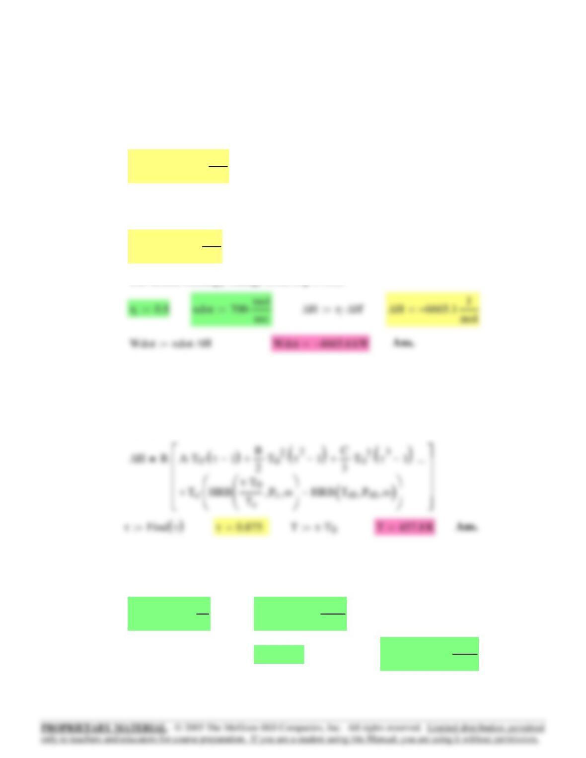
τ0.5:= (guess)
Given
∆SRAlnτ
()
⋅BT
τ
⋅D
T2
τ1+
2
⎛
⎜
⎝
⎞
⎠
⋅+
⎡
⎢
⎣
⎤
⎥
⎦
τ1−
()
⋅+ ln P
P0
⎛
⎜
⎝
⎞
⎠
−
⎡
⎢
⎣
⎤
⎥
⎦
⋅=
234

Tr0
T0
Tc
:= Tr0 1.282=Pr0
P0
Pc
:= Pr0 1.3706=
Pr
P
Pc
:= Pr0.137=
The entropy change is given by Eq. (6.92) combined with Eq. (5.15) with D = 0:
τ0.5:= (guess)
Given
∆SRAlnτ
()
⋅BT
0
⋅CT
02
⋅τ1+
2
⎛
⎜
⎝
⎞
⎠
⋅+
⎡
⎢
⎣
⎤
⎥
⎦τ1−
()
⋅+ ln P
P0
⎛
⎜
⎝
⎞
⎠
−
SRB τT0
⋅
Tc
Pr
,ω,
⎛
⎜
⎝
⎞
⎠SRB Tr0 Pr0
,ω,
()
−+
…
⎡
⎢
⎢
⎢
⎢
⎣
⎤
⎥
⎥
⎥
⎥
⎦
⋅=
Eq. (7.21) also applies to expansion:
7.22 Isobutane: Tc408.1 K⋅:= Pc36.48 bar⋅:= ω 0.181:=
T0523.15 K⋅:= P05000 kPa⋅:= P 500 kPa⋅:=
∆S0J
mol K⋅
⋅:= For the heat capacity of isobutane:
A 1.677:= B37.853 10 3−
⋅
K
:= C11.945−10 6−
⋅
K2
:=
235
Sliq 0.6493 kJ
kg K⋅
⋅:=x20.95:=
At 10 kPa:
S16.5138 kJ
kg K⋅
⋅:=H12851.0 kJ
kg
⋅:=
From Table F.2 @ 1700 kPa & 225 degC:7.23
Given
(guess)
τ0.7:=
The actual final temperature is now found from Eq. (6.91) combined with E
q
(4.7), written:
The actual enthalpy change from Eq. (7.16):
∆H’ 8331.4−J
mol
=
∆H’ ∆Hig RT
c
⋅HRB TrPr
,ω,
()
HRB Tr0 Pr0
,ω,
()
−
()
⋅+:=
∆Hig 11.078−kJ
mol
=
∆Hig R ICPH T0T,1.677,37.853 10 3−
⋅, 11.945−10 6−
⋅, 0.0,
()
⋅:=
The enthalpy change is given by Eq. (6.91):
236

7.24 T0673.15 K⋅:= P08 bar⋅:= P 1 bar⋅:=
For isentropic expansion, ∆S0J
mol K⋅
⋅:=
For the heat capacity of carbon dioxide:
A 5.457:= B1.045 10 3−
⋅
K
:= D 1.157−105
⋅K2
⋅:=
For the entropy change of an ideal gas, combine Eqs. (5.14) & (5.15) with C = 0:
τ0.5:= (guess)
Given
∆SRAlnτ
()
⋅BT
0
⋅D
T0τ⋅
()
2
τ1+
2
⎛
⎜
⎝
⎞
⎠
⋅+
⎡
⎢
⎣
⎤
⎥
⎦
τ1−
()
⋅+ ln P
P0
⎛
⎜
⎝
⎞
⎠
−
⎡
⎢
⎣
⎤
⎥
⎦
⋅=
τFind τ
()
:= τ 0.693=T’ τT0
⋅:= T’ 466.46 K=
Hliq 191.832 kJ
kg
⋅:= Hvap 2584.8 kJ
kg
⋅:= Svap 8.1511 kJ
kg K⋅
⋅:=
mdot 0.5 kg
sec
⋅:= Wdot 180−kW⋅:=
(b) For isentropic expansion to 10 kPa, producing wet steam:
237

∆HSCp T1⋅P2
P1
⎛
⎜
⎝
⎞
⎠
R
Cp
1−
⎡
⎢
⎢
⎣
⎤
⎥
⎥
⎦
⋅
⎡
⎢
⎢
⎣
⎤
⎥
⎥
⎦
→
⎯
⎯⎯⎯⎯⎯⎯⎯⎯
⎯
:=
Eq. (7.22) Applies to expanders as
well as to compressors
Ideal gases with constant heat capacities
∆HCpT2T1−()⋅[]
→
⎯
⎯⎯⎯⎯
⎯
:=
Cp
3.5
4.0
5.5
4.5
2.5
⎛
⎜
⎜
⎜
⎜
⎜
⎝
⎞
⎟
⎟
⎟
⎠
R⋅:=
P2
1.2
2.0
3.0
1.5
1.2
⎛
⎜
⎜
⎜
⎜
⎜
⎝
⎞
⎟
⎟
⎟
⎠
:=
T2
371
376
458
372
403
⎛
⎜
⎜
⎜
⎜
⎜
⎝
⎞
⎟
⎟
⎟
⎠
:=
P1
6
5
10
7
4
⎛
⎜
⎜
⎜
⎜
⎜
⎝
⎞
⎟
⎟
⎟
⎠
:=
T1
500
450
525
475
550
⎛
⎜
⎜
⎜
⎜
⎜
⎝
⎞
⎟
⎟
⎟
⎠
:=
Vectors containing data for Parts (a) through (e):7.25
∆HRAT
0
⋅τ1−
()
⋅B
2T02
⋅τ
21−
()
⋅+ D
T0
τ1−
τ
⎛
⎜
⎝
⎞
⎠
⋅+
⎡
⎢
⎣
⎤
⎥
⎦
⋅=
Given
For the enthalpy change of an ideal gas, combine Eqs. (4.2) and (4.7)
with C = 0:
238
By Eq. (5.37), for adiabatic operation :
⎜
⎜
⎜
By Eq. (5.14):
T2 433.213 K=T2 T1 1 ηP2
P1
⎛
⎜
⎝
⎞
⎠
R
Cp
1−
⎡
⎢
⎢
⎣
⎤
⎥
⎥
⎦
⋅+
⎡
⎢
⎢
⎣
⎤
⎥
⎥
⎦
⋅:=
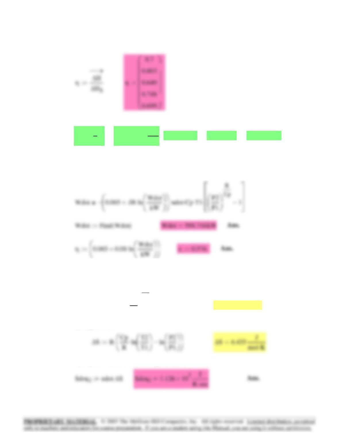
For an expander operating with an ideal gas with constant Cp, one can
show that:
⎜
⎜
⎜
⎜
⎜
⎢
⎢
⎥
⎥
Given
Wdot 600kW:=η 0.75:=
Guesses:
P2 1.2bar:=P1 6bar:=T1 550K:=ndot 175 mol
sec
:=Cp 7
2R⋅:=
7.26
⎜
239