120
CHAPTER 7
MULTIPLE REGRESSION
ANSWERS TO PROBLEMS AND CASES
2. The population of Y values is normally distributed about E(Y), the plane formed by the
3. The net regression coefficient measures the average change in the dependent variable per
6. a. A correlation matrix displays the correlation coefficients between every
possible pair of variables in the analysis.
7. a. Each variable is perfectly related to itself. The correlation is always 1.
121
b. The entries in a correlation matrix reflected about the main diagonal are the
8. a. Correlations:
Time Amount
The Full Model regression equation is:
Predictor Coef SE Coef T P VIF
Analysis of Variance
Source DF SS MS F P
The regression equation is
122
Predictor Coef SE Coef T P
Analysis of Variance
Source DF SS MS F P
c. Using the best model
f. Using the best model, the number of Items is not relevant so
g. Using the best model, the 95% prediction interval (interval forecast) for
123
9. a. Correlations: Food, Income, Size
Food Income
b. The regression equation is
When income is increased by one thousand dollars holding family size constant, the
c. Multicollinearity is a problem as indicated by VIF about 4.0. Size should be
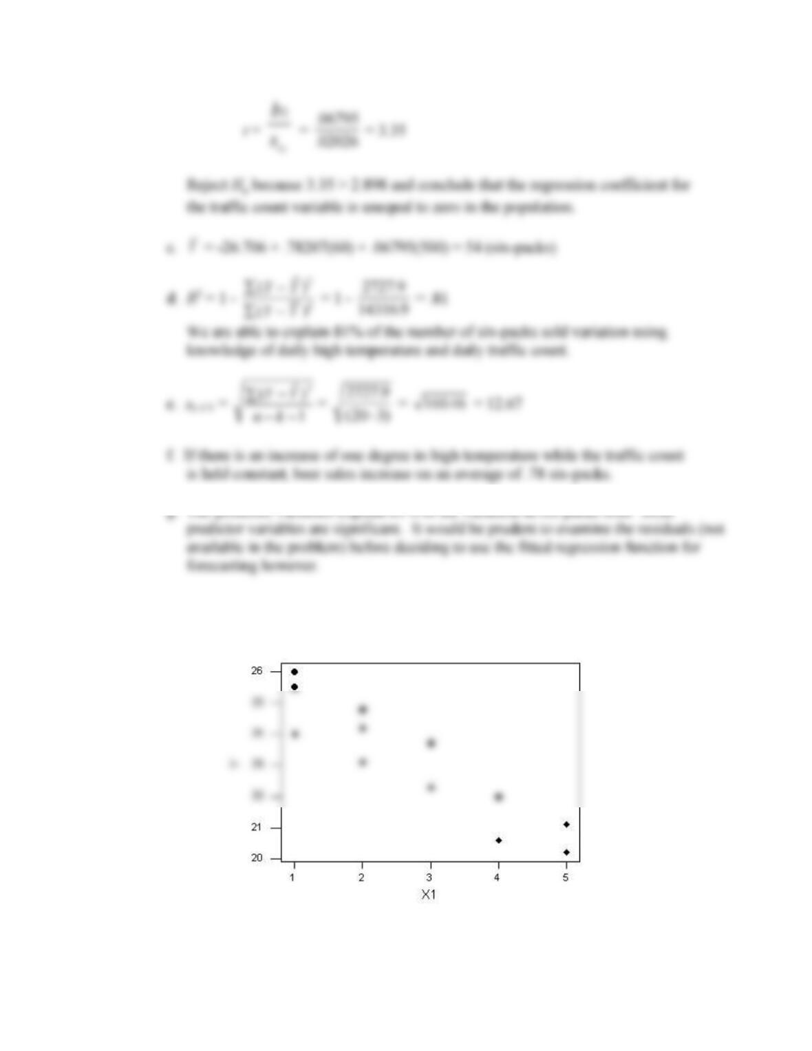
10. a. Both high temperature and traffic count are positively related to number of six-
. b. Reject
0:
10
H
if |t| > 2.898
124
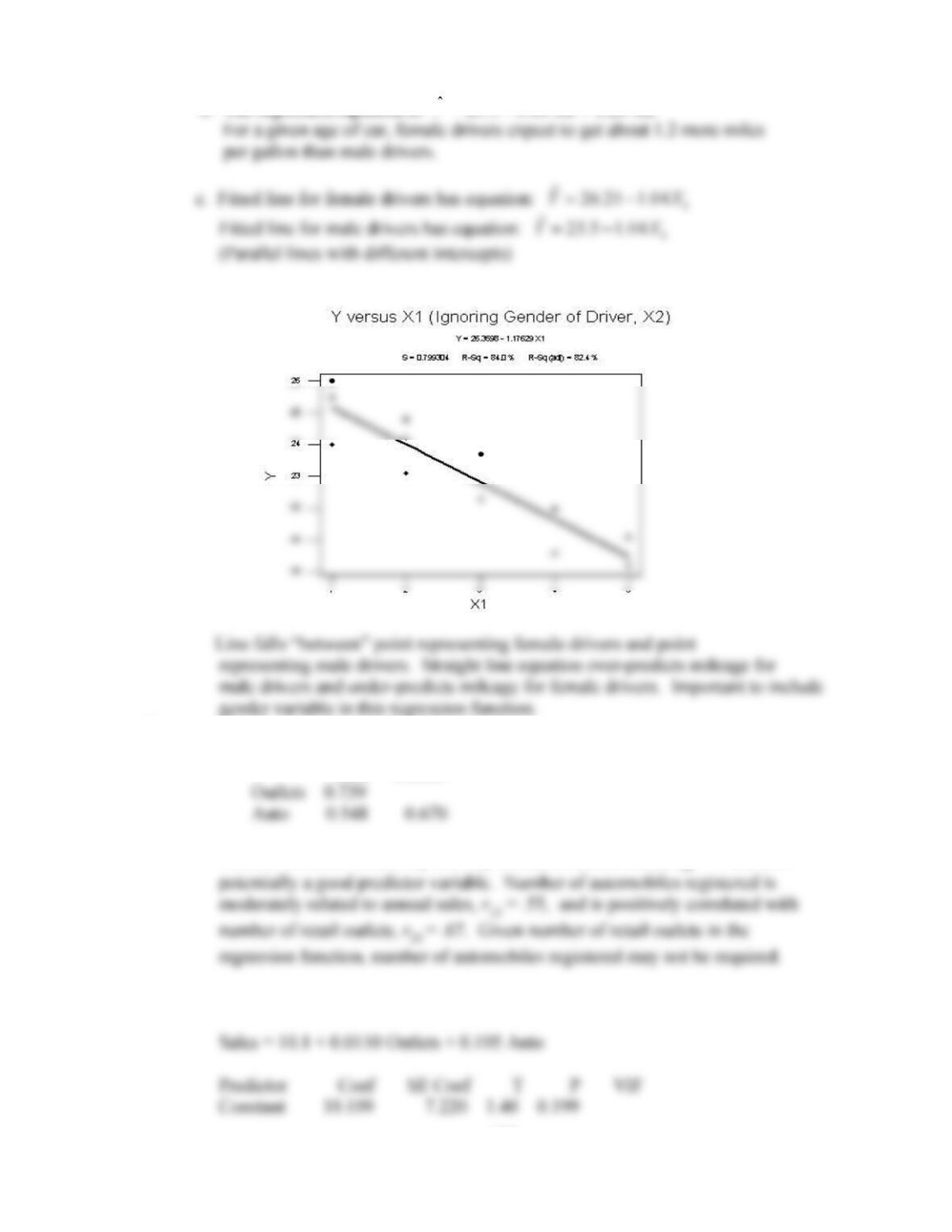
11. a. Scatter diagram follows. Female drivers indicated by solid circles, male divers by
diamonds.
125
b. The regression equation is:
Y
= 25.5 – 1.04 X1 + 1.21 X2
d.
12. a. Correlations: Sales, Outlets, Auto
Sales Outlets
Number of retail outlets is positively related to annual sales, r12 = .74, and is
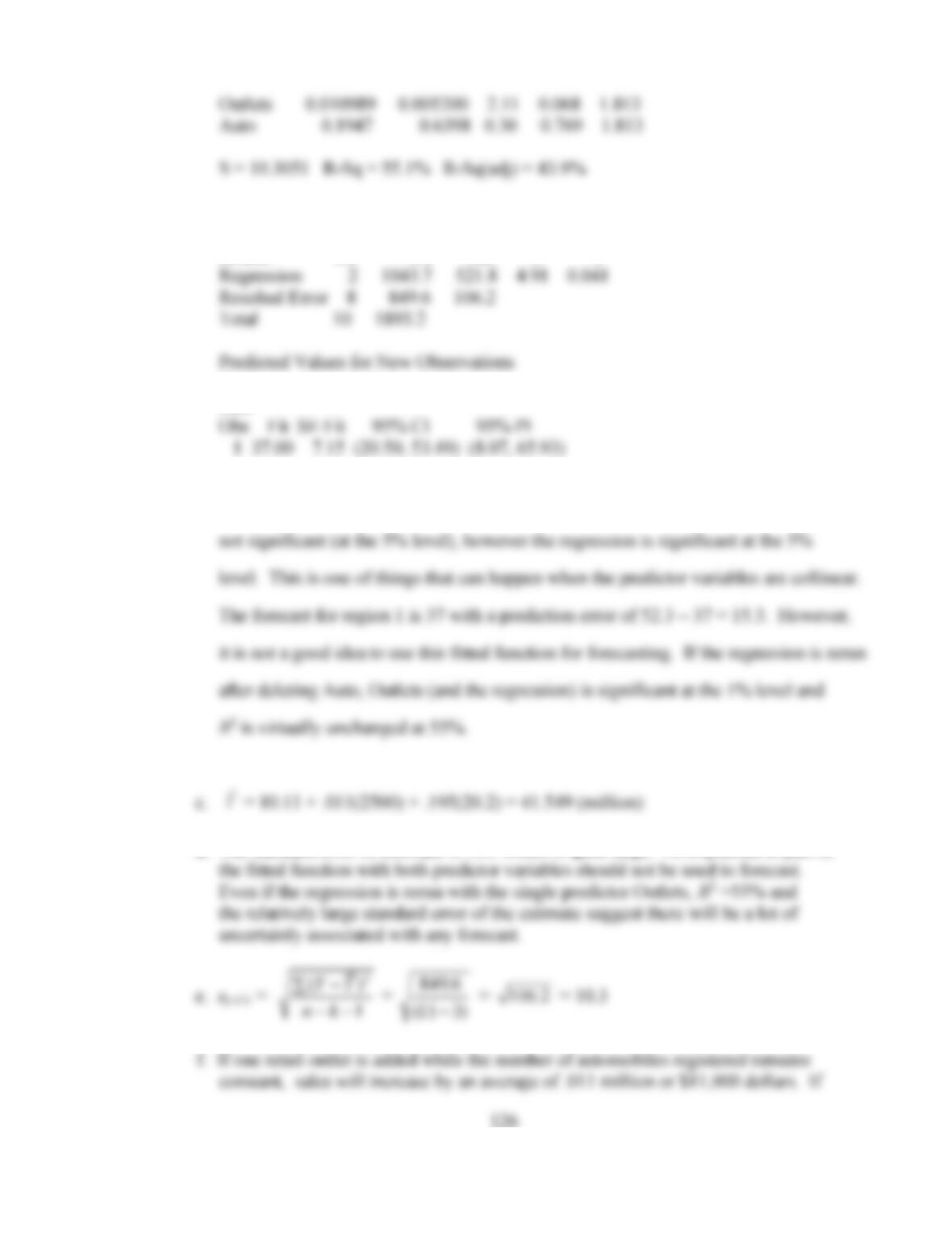
b. The regression equation is
Analysis of Variance
Source DF SS MS F P
New
As can be seen from the regression output, it appears as if each predictor variable is
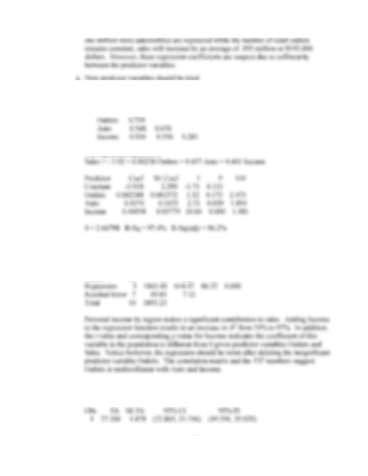
d. The standard error of estimate is 10.3 which is quite large. As explained in part b,
127
13. a. Correlations: Sales, Outlets, Auto, Income
Sales Outlets Auto
The regression equation is
Analysis of Variance
Source DF SS MS F P
b. Predicted Values for New Observations
New
128
Values of Predictors for New Observations
New
Obs Outlets Auto Income
c. The standard error of estimate has been reduced to 2.67 from 10.3 and R2 has increased
d. The best choice is to drop Outlets from the regression function. If this is done,
the regression equation is
14. a. Reject H0 : 1 = 0 if |t |> 3.1.
b. If the effort index increases one point while aptitude test score remains constant,
129
( )
Y Y
2
.
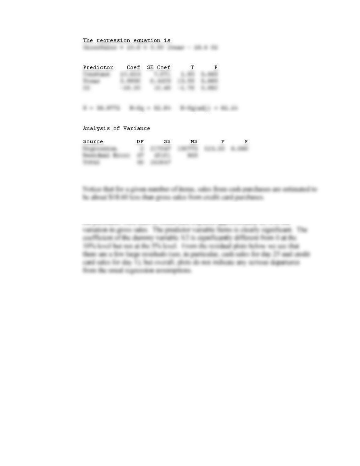
15. a. Scatter plot for cash purchases versus number of items (rectangles) and credit card
purchases versus number of items (solid circles) follows.
b. Minitab regression output:
130
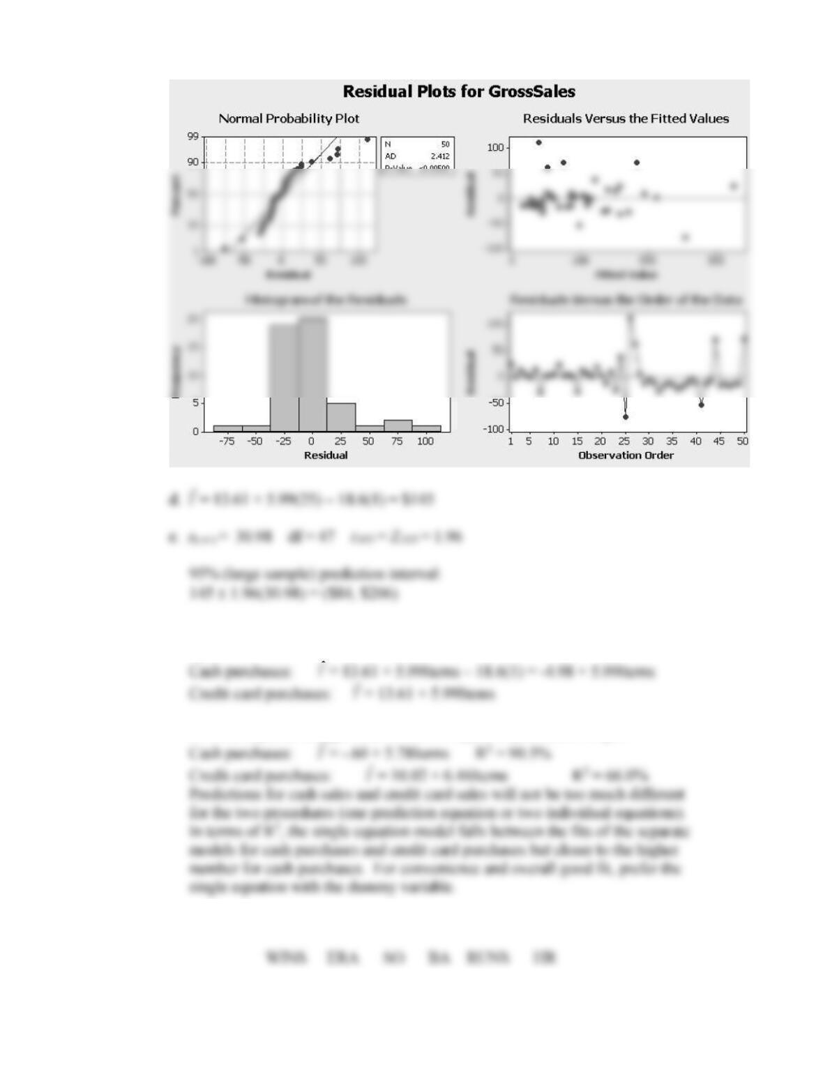
c. The regression in part b is significant. The number of items sold and whether
131
f. Fitted function in part b is effectively two parallel straight lines given by the
equations:
If we fit separate straight lines to the two types of purchases we get:
16. a. Correlations: WINS, ERA, SO, BA, RUNS, HR, SB
ERA is moderately negatively correlated with WINS.
SO is essentially uncorrelated with WINS.
b. The stepwise results are the same for an alpha to enter = alpha to remove = .05 or
.15 (the Minitab default) or F to remove = F to enter =4.
Response is WINS on 6 predictors, with N = 26
RUNS 0.087 0.115
ERA -18.0
17. a. View will enter the stepwise regression function first since it has the largest
correlation with Price. After that the order of entry is difficult to determine from