Fluid Flow in Soils and Rock Chapter 7
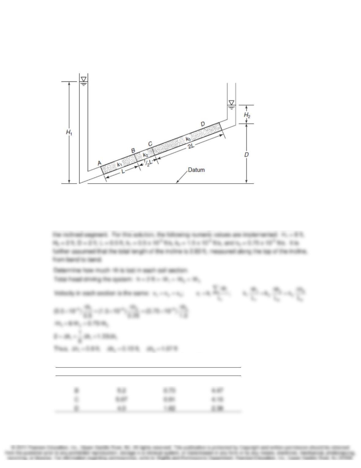
7-18. An inclined permeameter tube is filled with three layers of soil of different permeabilities as
in Fig. P7.18. Express the head at points A, B, C, and D (with respect to the datum indicated) in
terms of the different dimensions and permeabilities. (After A. Casagrande.)
SOLUTION:
The problem cannot be readily solved without some additional assumptions. The following
solution is presented assuming the tube is inclined at an angle of 45o and the soil is centered in
pe
Use the datum and trigonometry to determine h, h ,and h .
Point h (ft) he (ft) hp (ft)
A 6 0.38 5.62
Fluid Flow in Soils and Rock Chapter 7
7-19. Assume the soil of Fig. 7.10 has a saturated density of 1.89 Mg/m3. If the head of water h
above elevation B is 2.45 m, compute the effective stress at elevation A at the bottom of the soil
sample during flow. What is the effective stress under these conditions at midheight in the soil
column during steady-state flow?
SOLUTION:
33222
‘ at Elev. A (bottom of soil sample)
(5 m)(1.89 Mg m ) (2 m)(1.0 Mg m ) (9.81m s ) (11.45 Mg m )(9.81m s ) 112.32 kPa
σ
⎡⎤
σ= + = =
⎣⎦
7-20. The foundation soil at the toe of a masonry dam has a porosity of 38% and a
ρ
s of 2.73
Mg/m3. To assure safety against piping, the specifications state that the upward gradient must not
exceed 30% of the gradient at which a quick condition occurs. What is the maximum permissible
upward gradient? (After Taylor, 1948.)
SOLUTION:
n0.38
e 0.613
1n 10.38
== =
−−
Fluid Flow in Soils and Rock Chapter 7
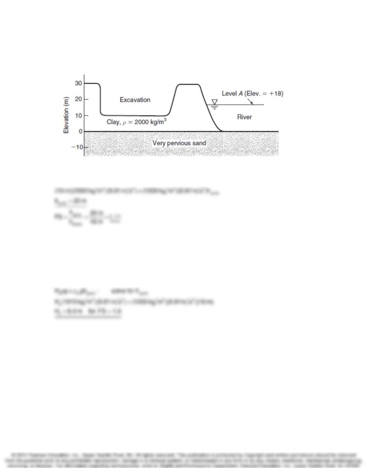
7-23. A contractor plans to dig an excavation as show in Fig. P7.23. If the river is at level A, what
is the factor of safety against quick conditions? Neglect any vertical shear. To what elevation can
the water rise before a quick condition will develop? (After D. N. Humphrey.)
SOLUTION:
s w quick quick
H g gh : solve for h
ρ=ρ
7-24. Given the excavation as shown in Example 7.13, with h = 18 m and
ρ
= 1915 kg/m3.
Calculate the minimum allowable Hs.
SOLUTION:
Fluid Flow in Soils and Rock Chapter 7
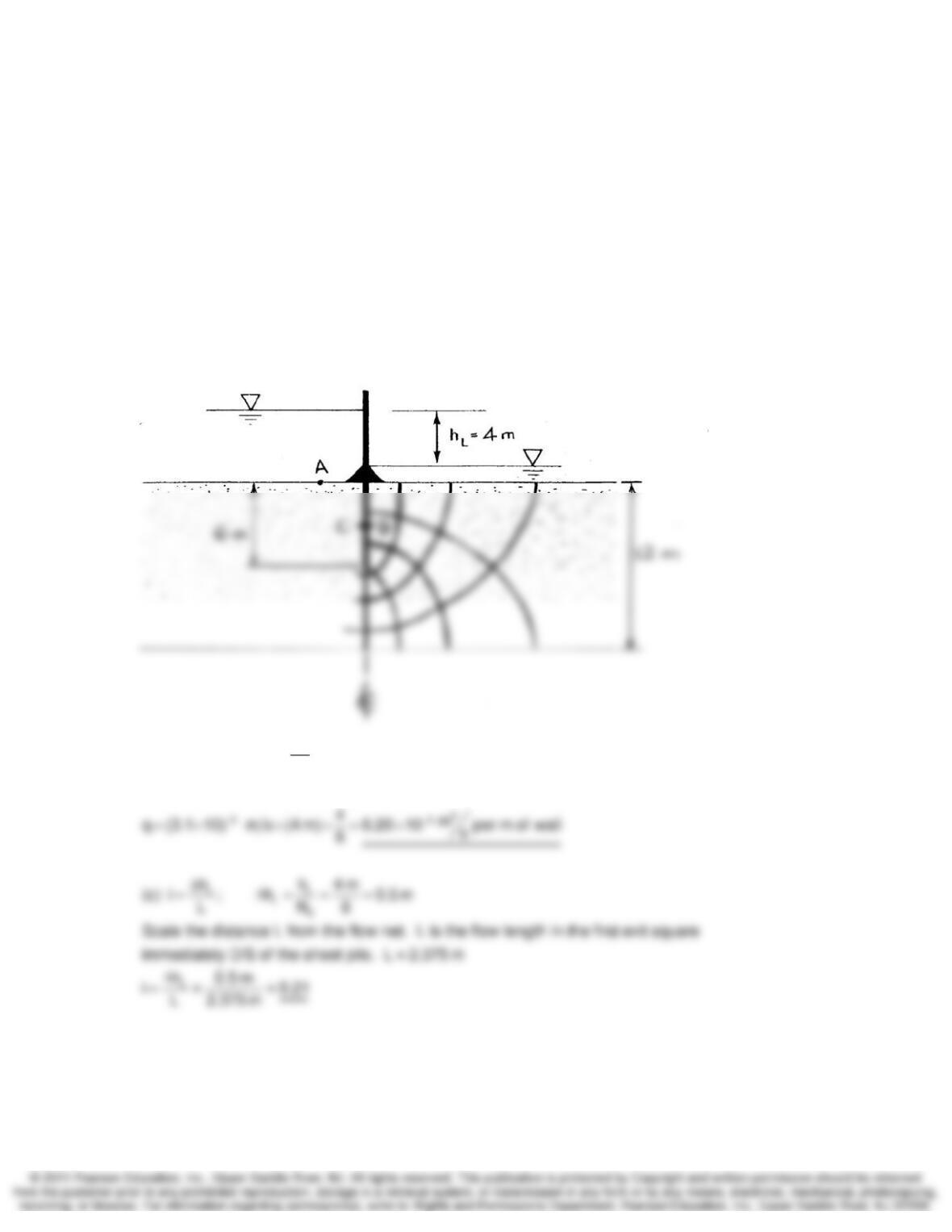
7-25. A sheet pile wall has been installed partially through a silty sand layer, similar to the one
shown in Fig. 7.13(b). Assume a sheet pile 12 m long penetrates 6 m (halfway) into the silty sand
layer of thickness 12 m. For this condition: (a) Draw a flow net using three (or four at most) flow
channels. Note that the flow net is completely symmetrical about the bottom of the sheet pile.
(This part is needed for the solution of Problem 7.35.) (b) If the water height on the upstream
side is 5 m and on the downstream side 1 m, compute the amount of water flowing under the
sheet pile per meter of wall if the coefficient of permeability is 3.1 x 10⁻⁴ cm/s. (c) Compute the
maximum hydraulic gradient at the downstream side of the sheet pile.
SOLUTION:
(a) The sketch below contains a ‘5-minute’ flow net that is symmetric about a vertical axis through
the sheet pile.
f
L
d
fd L
N
(b) Eq. 7.20: q kh N
From the flow net: N 4, N 4 2 8, h 5 1 4 m
=
= =×= =−=

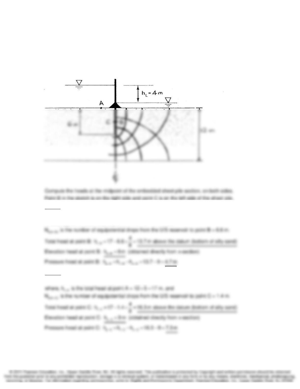
7-26. Using the data of Fig. 7.16, compute the total head, piezometric head, pressure head, and
elevation head for points C and C’. Assume any convenient datum.
SOLUTION:
tC t@U/S d(U/SC) L
Assume a datum at the elevation of the impervious boundary.
Total head at point C: h h N h
−−
=− ×Δ
Fluid Flow in Soils and Rock Chapter 7
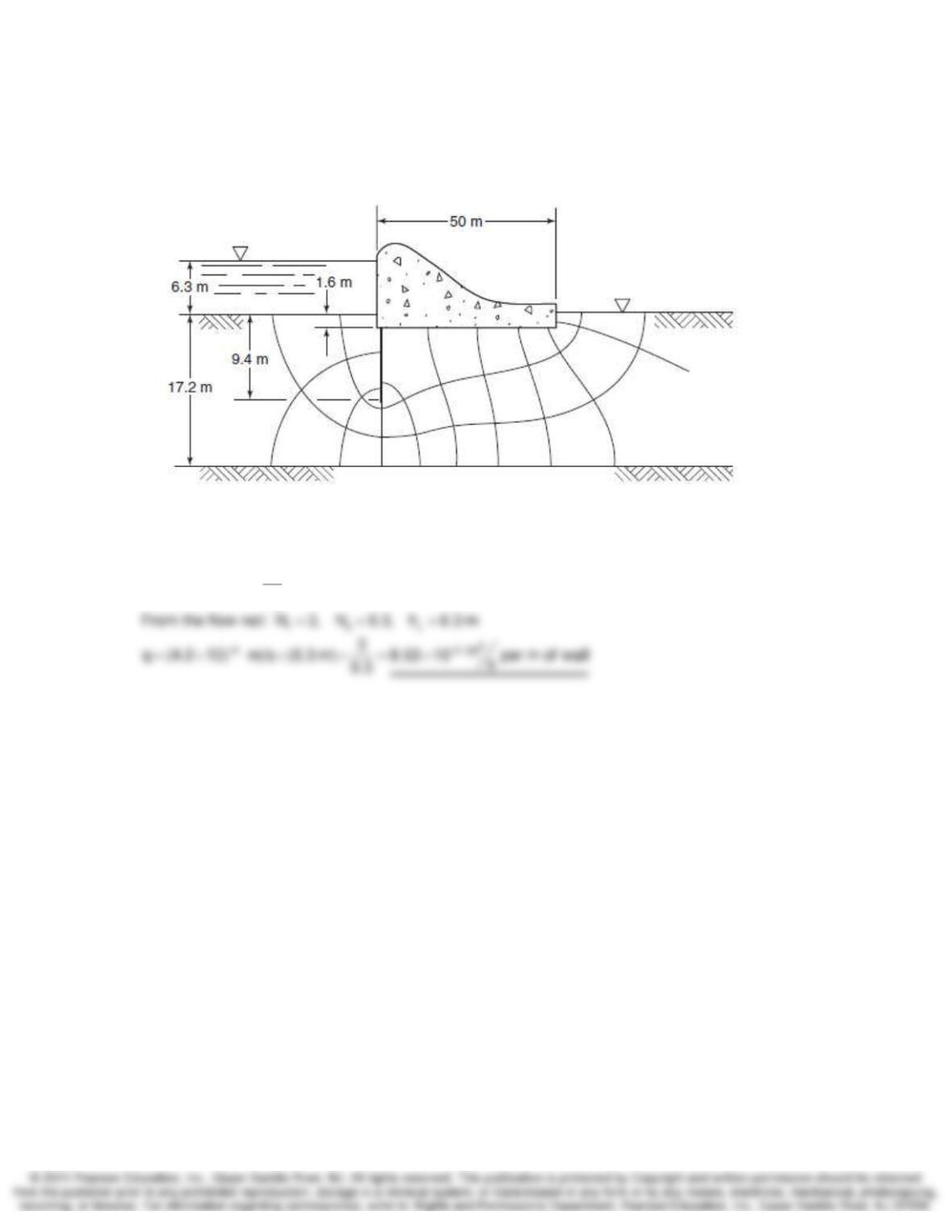
7-27. Assuming that you have completed the flow net of Problem 7.24, compute the total head,
piezometric head, pressure head, and elevation head for a point halfway up the sheet pile from its
base, on either side of the sheet pile. Assume the datum is at the bottom of the silty sand layer.
Plot gradient versus depth of piling and extrapolate to find the exit gradient.
SOLUTION:
Point B
Total head at mid tB tA d(AB) L
tA
point (B): h h N h
where, h is the total head at point A = 12 5 17 m, and
−− −
−
=− ×Δ
+=
Point C
Total head at
tC tA d(AC) L
midpoint (C): h h N h
−− −
=− ×Δ
Fluid Flow in Soils and Rock Chapter 7
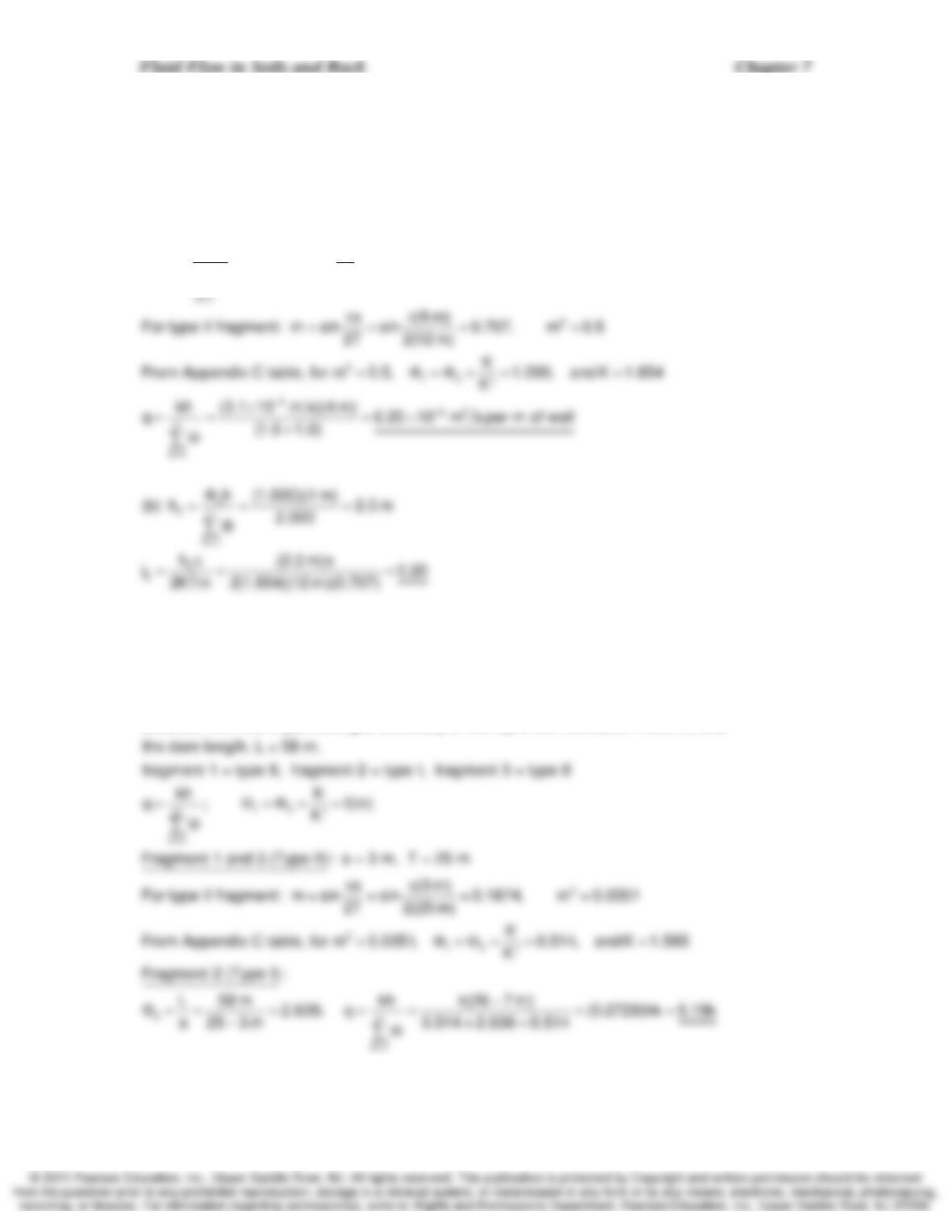
7-30. For the completed flow net of Fig. P7.30, compute the flow under the dam per meter of
dam if the coefficient of permeability is 4.2 x 10⁻⁴ cm/s.
SOLUTION:
f
L
d
N
Eq. 7.20: q kh N
=
7-31. Given the data of Problem 7.25. Using the method of fragments, determine: (a) The
amount of water flowing under the sheet pile per meter of wall. (b) The exit gradient.
SOLUTION:
12
n
Divide the flow regime into two fragments by drawing a vertical line at the sheet pile.
Both fragments are type II. s = 6 m, T = 12 m
kh K
(a) q ; f(m)
K’
=Φ=Φ==
Φ
∑
7-32. For the dam of Fig. 7.15, solve for q using the method of fragments.
SOLUTION:
Divide flow regime into 3 fragments by drawing vertical lines at U/S and D/S ends of the dam.
Assume all dimensions in Fig. 7.15 are in meters. The dam embedment depth = 3 m.
Distance from the impe
rvious geo-boundary to the top of the foundation is 25 m, and
Fluid Flow in Soils and Rock Chapter 7
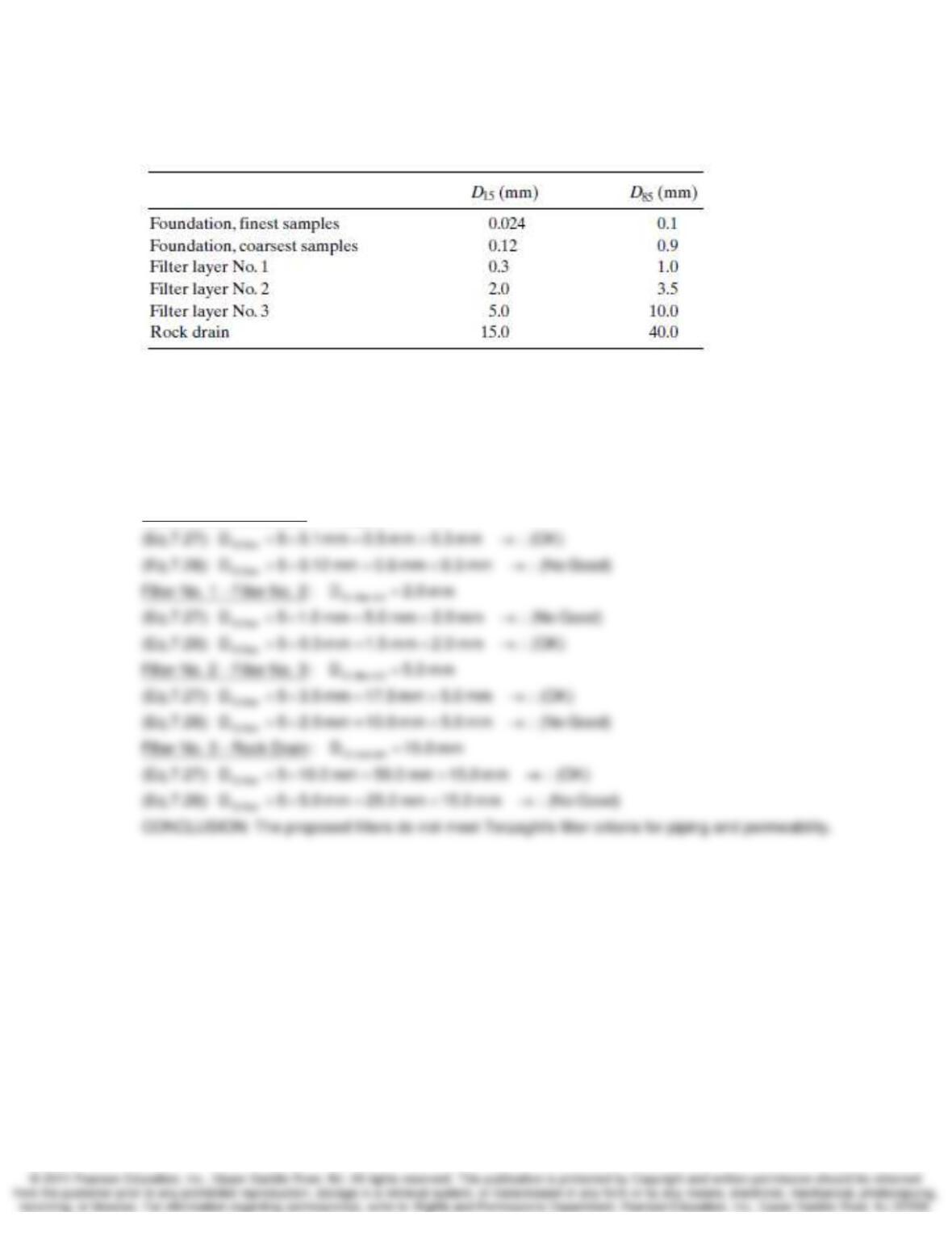
7-37. A protective three-layer filter is proposed between the foundation and rock drain located
near the toe of a compacted earth-fill dam. Is this filter acceptable?
SOLUTION:
15 filter 85 soil
Use Terzaghi‘s criteria for piping (Eq. 7.27) and permeability (Eq. 7.28) to evaluate
the acceptability of the proposed filters. Use FS = 5.
Eq.7.27 (piping): D (4 to 5)D and Eq.7.28 (permea<15 filter 15 soil
15 filter #1
bility): D (4 to 5)D
Foundation – Filter No. 1: D 0.3 mm
>
=
Fluid Flow in Soils and Rock Chapter 7
7-38. In an attempt to reduce minor surface instability and maintenance problems on the
backslopes of a rural highway, interceptor trench drains are to be installed at the top of the slope
of to intercept surface and infiltrating groundwater from the hillsides above the road. The drains
are 1 to 1.5 m deep, and the drainage trench lined with a geotextile filter. A perforated drain pipe
is placed in the bottom of the trench, and the trench is backfilled with coarse drainage aggregate.
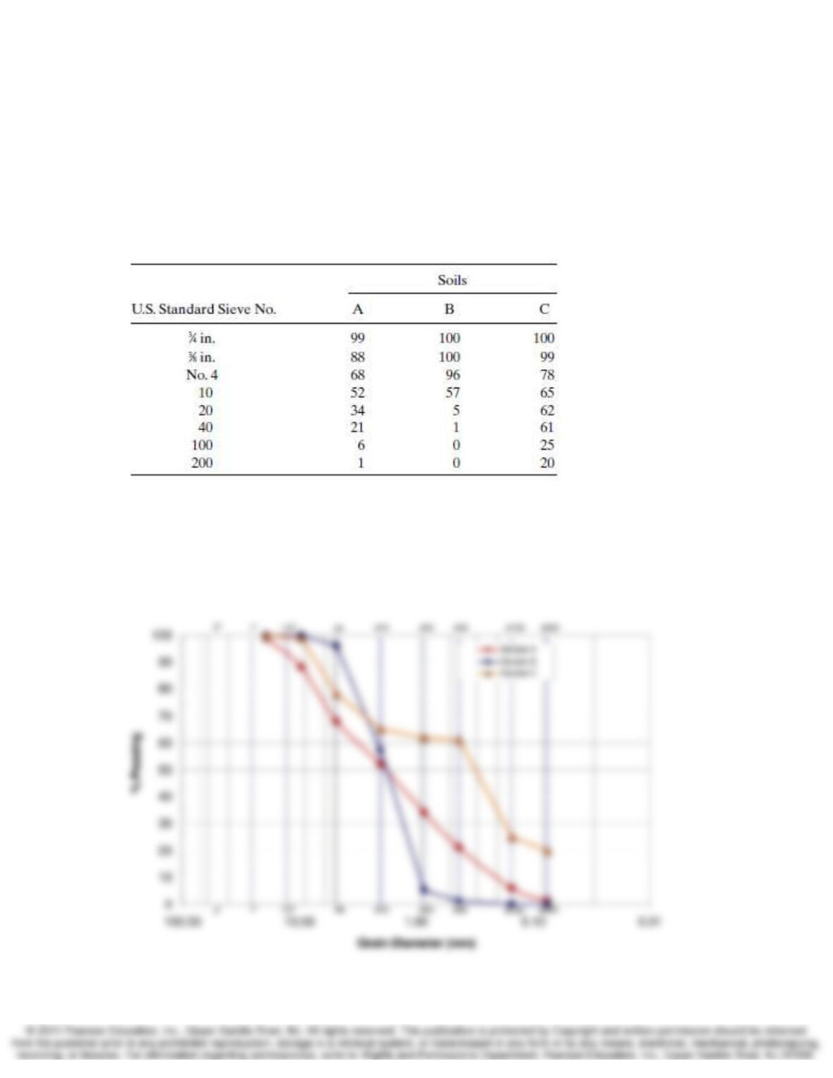
Sieve analyses were performed on samples of soils typical of the problem areas along the
highway alignment, and the following average data (percent passing) were obtained: Design the
geotextile filter for the interceptor drains.
SOLUTION:
Following are grain size distribution plots for the three soil samples. This information can be used
to design the geotextile filter using the FHWA filter design procedure outlined in Section 7.10.4
Grain Size Distribution Plot