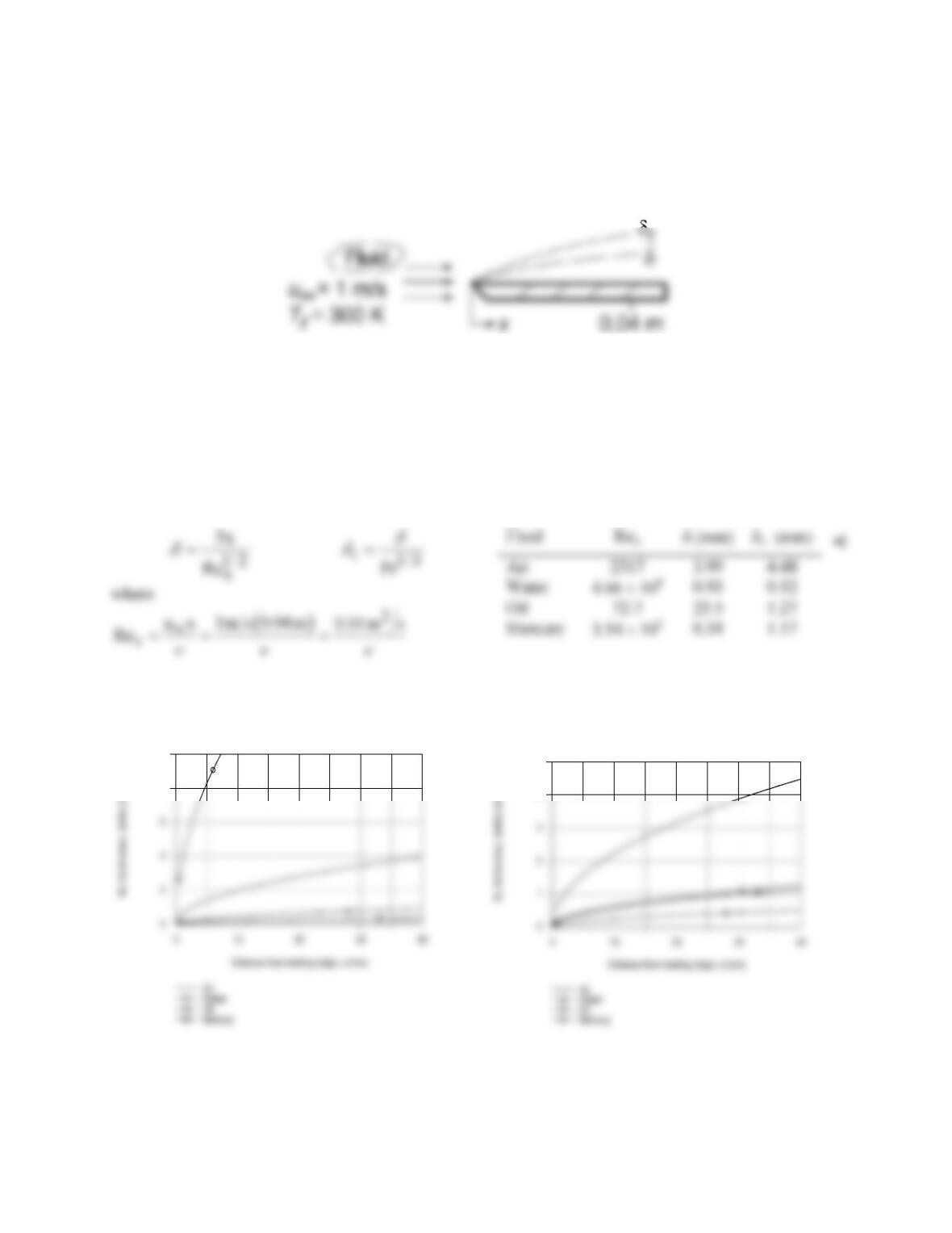
PROBLEM 7.1
KNOWN: Temperature and velocity of fluids in parallel flow over a flat plate.
FIND: (a) Velocity and thermal boundary layer thicknesses at a prescribed distance from the leading
edge, and (b) For each fluid plot the boundary layer thicknesses as a function of distance.
SCHEMATIC:
ASSUMPTIONS: (1) Transition Reynolds number is 5 × 10⁵.
PROPERTIES: Table A.4, Air (300 K, 1 atm): ν = 15.89 × 10⁻⁶ m2/s, Pr = 0.707; Table A.6, Water
(300 K): ν = µ/ρ = 855 × 10-6 N⋅s/m2/997 kg/m3 = 0.858 × 10⁻⁶ m2/s, Pr = 5.83; Table A.5, Engine Oil
(300 K): ν = 550 × 10-6 m2/s, Pr = 6400; Table A.5, Mercury (300 K): ν = 0.113 × 10⁻⁶ m2/s, Pr =
0.0248.
ANALYSIS: (a) If the flow is laminar, the following expressions may be used to compute δ and δt,
respectively,
(b) Using IHT with the foregoing equations, the boundary layer thicknesses are plotted as a function of
distance from the leading edge, x.
8
10
4
5
COMMENTS: (1) Note that δ ≈ δt for air, δ > δt for water, δ >> δt for oil, and δ < δt for mercury. As
expected, the boundary layer thicknesses increase with increasing distance from the leading edge.
(2) The value of δt for mercury should be viewed as a rough approximation since the expression for δ/δt
was derived subject to the approximation that Pr > 0.6.
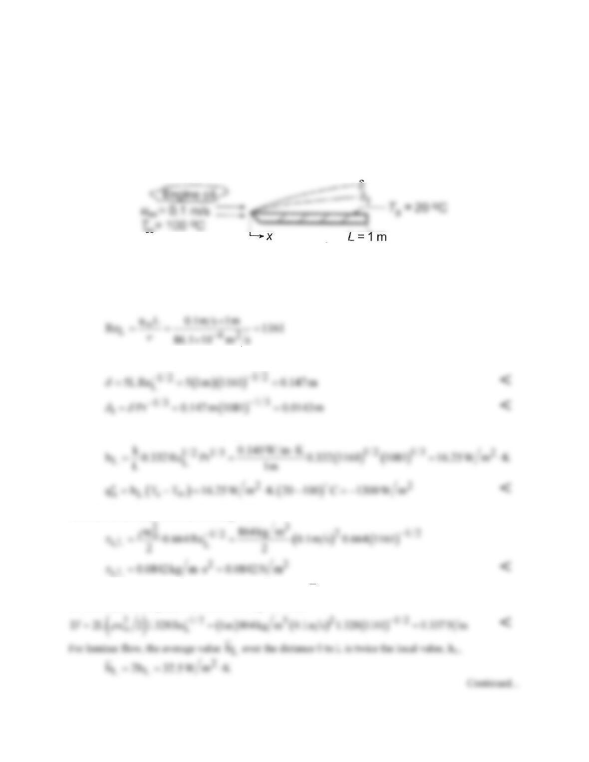
PROBLEM 7.2
KNOWN: Temperature and velocity of engine oil. Temperature and length of flat plate.
FIND: (a) Velocity and thermal boundary layer thickness at trailing edge, (b) Heat flux and surface
shear stress at trailing edge, (c) Total drag force and heat transfer rate per unit plate width, and (d) Plot
the boundary layer thickness and local values of the shear stress, convection coefficient, and heat flux as
a function of x for 0 ≤ x ≤ 1 m.
SCHEMATIC:
ASSUMPTIONS: (1) Critical Reynolds number is 5 × 10⁵, (2) Flow over top and bottom surfaces.
PROPERTIES: Table A.5, Engine Oil (Tf = 333 K): ρ = 864 kg/m3, ν = 86.1 × 10⁻⁶ m2/s, k = 0.140
W/m⋅K, Pr = 1081.
ANALYSIS: (a) Calculate the Reynolds number to determine nature of the flow,
Hence the flow is laminar at x = L. From Eqs. 7.19 and 7.24,
(b) The local convection coefficient, Eq. 7.23, and heat flux at x = L are
Also, the local shear stress is, from Eq. 7.20,
(c) With the drag force per unit width given by
s,L
D 2L
τ
′=
where the factor of 2 is included to account
for both sides of the plate, it follows from Eq. 7.29 that
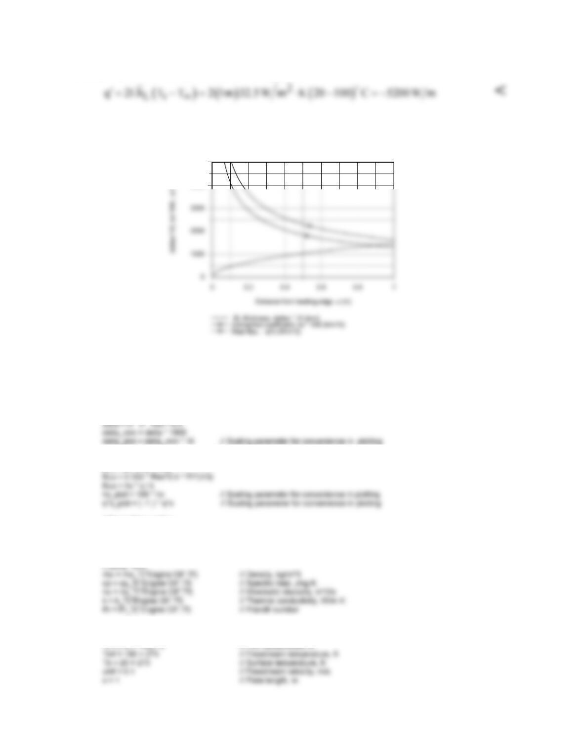
PROBLEM 7.2 (Cont.)
The total heat transfer rate per unit width of the plate is
(d) Using IHT with the foregoing equations, the boundary layer thickness, and local values of the
convection coefficient and heat flux were calculated and plotted as a function of x.
4000
5000
COMMENTS: (1) Note that since Pr >> 1, δ >> δt. That is, for the high Prandtl liquids, the velocity
boundary layer will be much thicker than the thermal boundary layer.
(2) A copy of the IHT Workspace used to generate the above plot is shown below.
// Boundary layer thickness, delta
// Convection coefficient and heat flux, q”x
q’‘x = hx * (Ts – Tinf)
// Reynolds number
Rex = uinf * x / nu
// Properties Tool: Engine oil
// Engine Oil property functions : From Table A.5
// Assigned variables
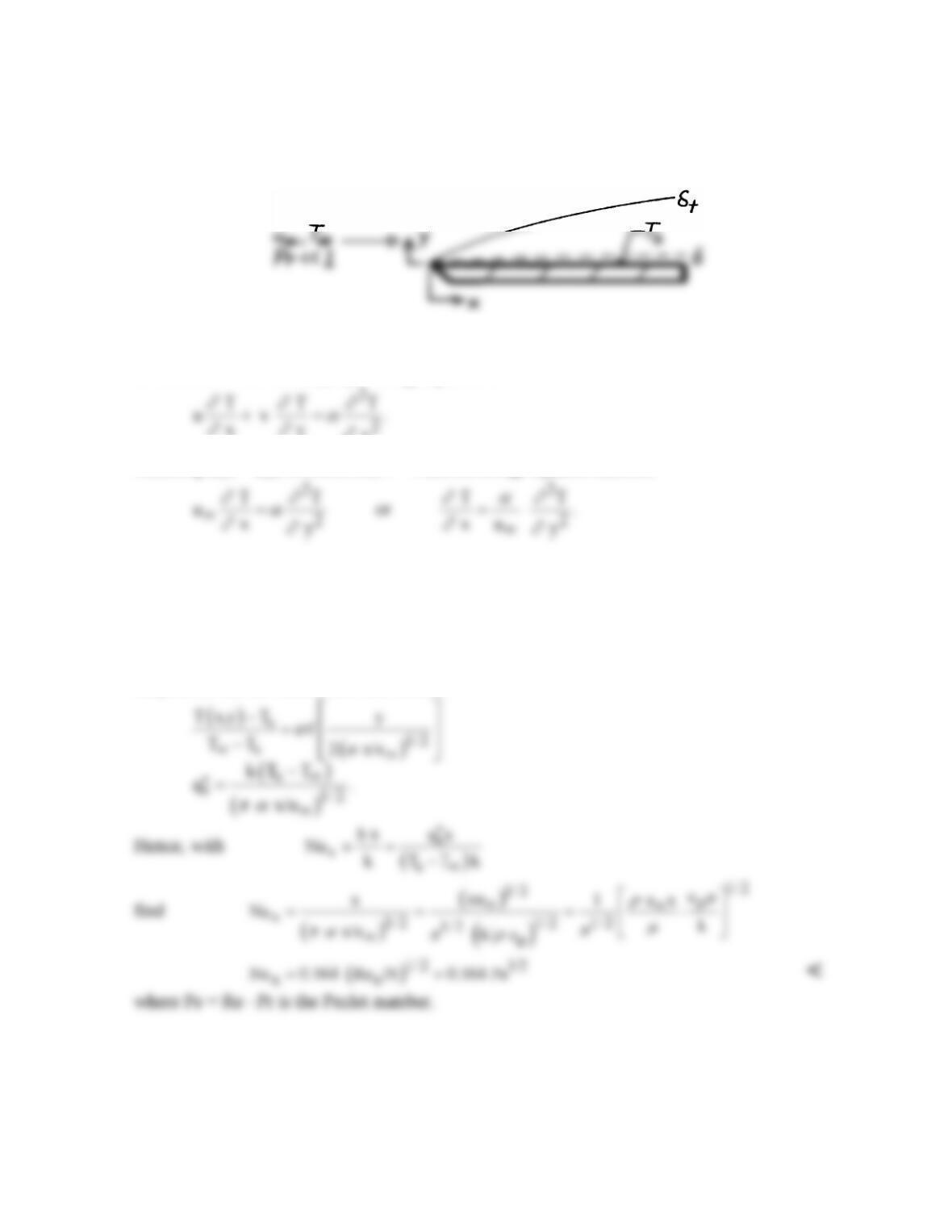
PROBLEM 7.3
KNOWN: Liquid metal in parallel flow over a flat plate.
FIND: An expression for the local Nusselt number.
SCHEMATIC:
ASSUMPTIONS: (1) Steady, incompressible flow, (2) δ << δt, hence u(y) ≈ u∞, (3) Boundary layer
approximations are valid, (4) Constant properties.
ANALYSIS: The boundary layer energy equation is
x y
y
∂∂
∂
Assuming u(y) = u∞, it follows that v = 0 and the energy equation becomes
Boundary Conditions: T(x,0) = Ts, T(x,∞) = T∞.
Initial Condition: T(0,y) = T∞.
The differential equation is analogous to that for transient one-dimensional conduction in a plane
wall, and the conditions are analogous to those of Fig. 5.7, Case (1). Hence the solution is given by
Eqs. 5.60 and 5.61. Substituting y for x, x for t, T∞ for Ti, and α/u∞ for α, the boundary layer
temperature and the surface heat flux become
COMMENTS: Because k is very large, axial conduction effects may not be negligible. That is, the
α ∂2T/∂x2 term of the energy equation may be important.
PROBLEM 7.4
KNOWN: Form of velocity profile for flow over a flat plate.
FIND: (a) Expression for profile in terms of u∞ and δ, (b) Expression for δ(x), (c) Expression for
Cf,x.
ASSUMPTIONS: (1) Steady state conditions, (2) Constant properties, (3) Incompressible flow, (4)
Boundary layer approximations are valid.
ANALYSIS: (a) From the boundary conditions
∞
(b)From the momentum integral equation for a flat plate
Separating and integrating, find
y0
=
and the friction coefficient is
COMMENTS: The foregoing results underpredict those associated with the exact solution
()
-1/2 -1/2
x f,x x
4.96 x Re , C 0.664 Re
δ
= =
and the cubic profile
(
1/2
x
4.64 x Re ,
δ
−
=
)
1/2
f,x x
C 0.646 Re .
−
=
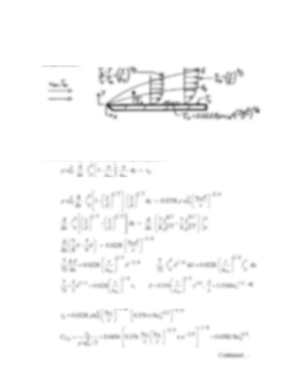
PROBLEM 7.5
KNOWN: Velocity and temperature profiles and shear stress-boundary layer thickness
relation for turbulent flow over a flat plate.
FIND: (a) Expressions for hydrodynamic boundary layer thickness and average friction
coefficient, (b) Expressions for local and average Nusselt numbers.
ASSUMPTIONS: (1) Steady flow, (2) Constant properties, (3) Fully turbulent boundary
layer, (4) Incompressible flow, (5) Isothermal plate, (6) Negligible viscous dissipation, (7) δ ≈
δt.
ANALYSIS: (a) The momentum integral equation is
Substituting the expression for the wall shear stress
Knowing δ, it follows
PROBLEM 7.5 (Cont.)
The average friction coefficient is then
(b) The energy integral equation for turbulent flow is
pp
Hence,
Hence, with
1/5
x
1 and /x 0.376 Re ,
ξδ
−
≈=
k
Hence,
COMMENTS: (1) The foregoing results are in excellent agreement with empirical
correlations, except that use of Pr1/3 instead of Pr, would be more appropriate. This result
arose because of the assumption
t
δ≈δ
, which is only valid for Pr ≈ 1.
(2) Note that the 1/7 profile breaks down at the surface. For example,
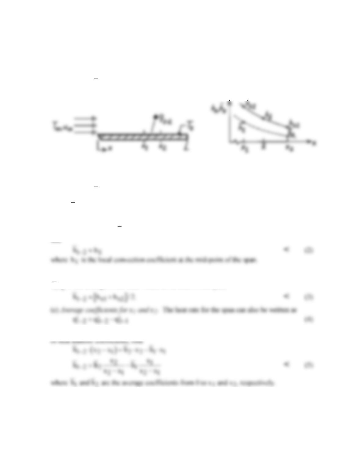
PROBLEM 7.6
KNOWN: Parallel flow over a flat plate and two locations representing a short span x1 to x2
where (x2 – x1) << L.
FIND: Three different expressions for the average heat transfer coefficient over the short
span x1 to x2,
12
h.
−
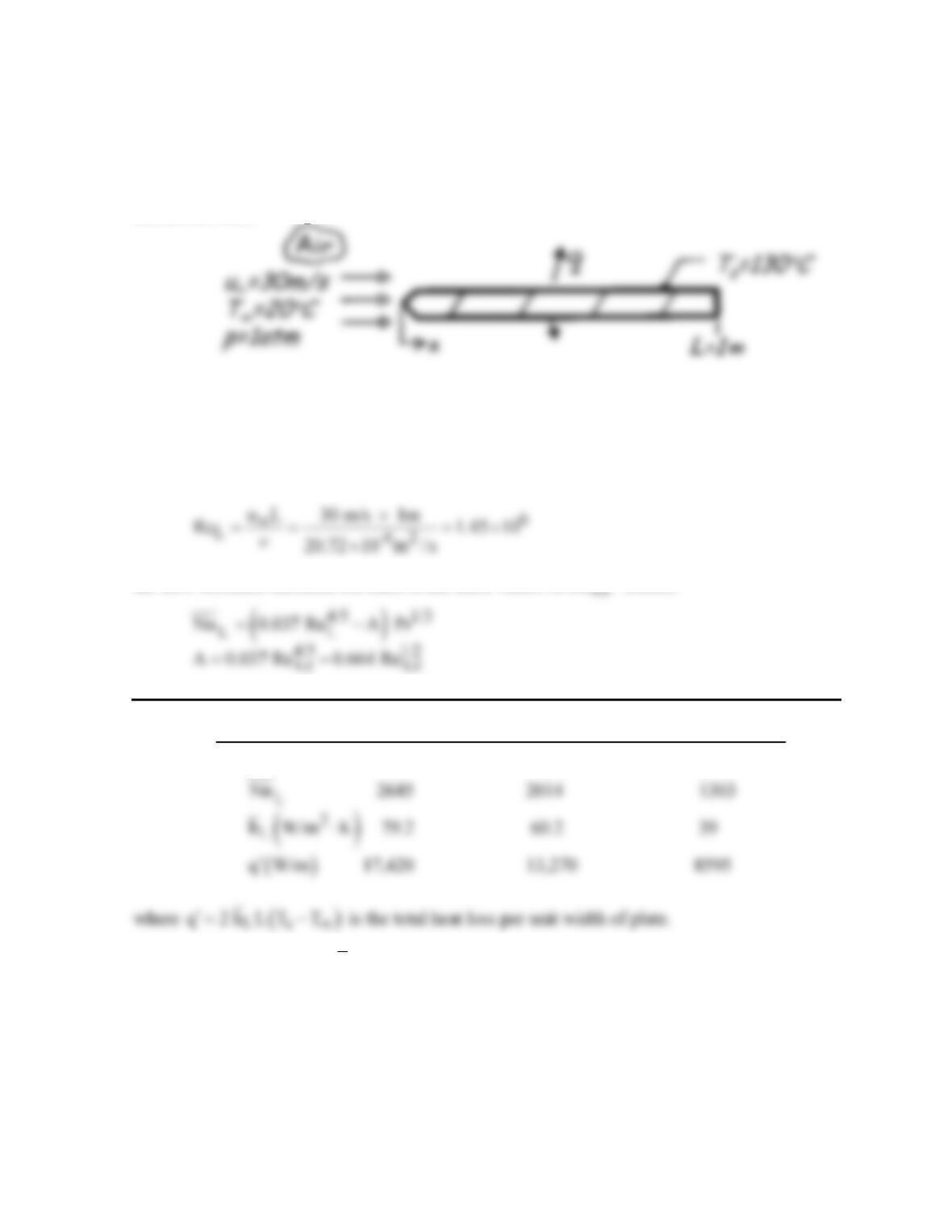
SCHEMATIC:
ASSUMPTIONS: (1) Parallel flow over a flat plate.
ANALYSIS: The heat rate per unit width for the span can be written as
( )( )
12 12 2 1 s
q h x xTT
−− ∞
′= −−
(1)
where
12
h−
is the average heat transfer coefficient over the span and can be evaluated in
either of the following three ways:
(a) Local coefficient at
( )
12
x x x / 2.= +
If the span is very short, it is reasonable to assume
that
(b) Local coefficients at x1 and x2. If the span is very short it is reasonable to assume that
h
1 2−
is the average of the local values at the ends of the span,
where the rate q0-x denotes the heat rate for the plate over the distance from 0 to x. In terms
COMMENTS: Eqs. (2) and (3) are approximate and work better when the span is small and
the flow is turbulent rather than laminar (hx ~ x-0.2 vs hx ~ x-0.5). Of course, we require that
xc < x1, x2 or xc > x1, x2; that is, the approximations are inappropriate around the transition
region. Eq. (5) is an exact relationship, which applies under any conditions.
PROBLEM 7.7
KNOWN: Speed and temperature of atmospheric air flowing over a flat plate of prescribed
length and temperature.
FIND: Rate of heat transfer corresponding to Rex,c = 105, 5 × 10⁵ and 106.
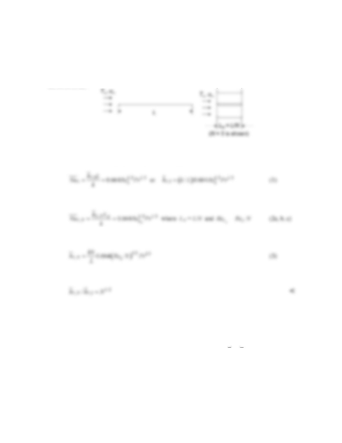
SCHEMATIC:
ASSUMPTIONS: (1) Flow over top and bottom surfaces.
PROPERTIES: Table A-4, Air (Tf = 348K, 1 atm): ρ = 1.00 kg/m3, ν = 20.72 × 10⁻⁶ m2/s,
k = 0.0299 W/m⋅K, Pr = 0.700.
ANALYSIS: With
the flow becomes turbulent for each of the three values of Rex,c. Hence,
Rex,c 105 5×10⁵ 106
A 160 871 1671
COMMENTS: Note that
L
h
decreases with increasing Rex,c, as more of the surface
becomes covered with a laminar boundary layer.
PROBLEM 7.8
KNOWN: Length of isothermal flat plate in parallel flow, L.
FIND: Expression for the average heat transfer coefficients for N plates each of length LN = L/N to
the average coefficient for the single plate.
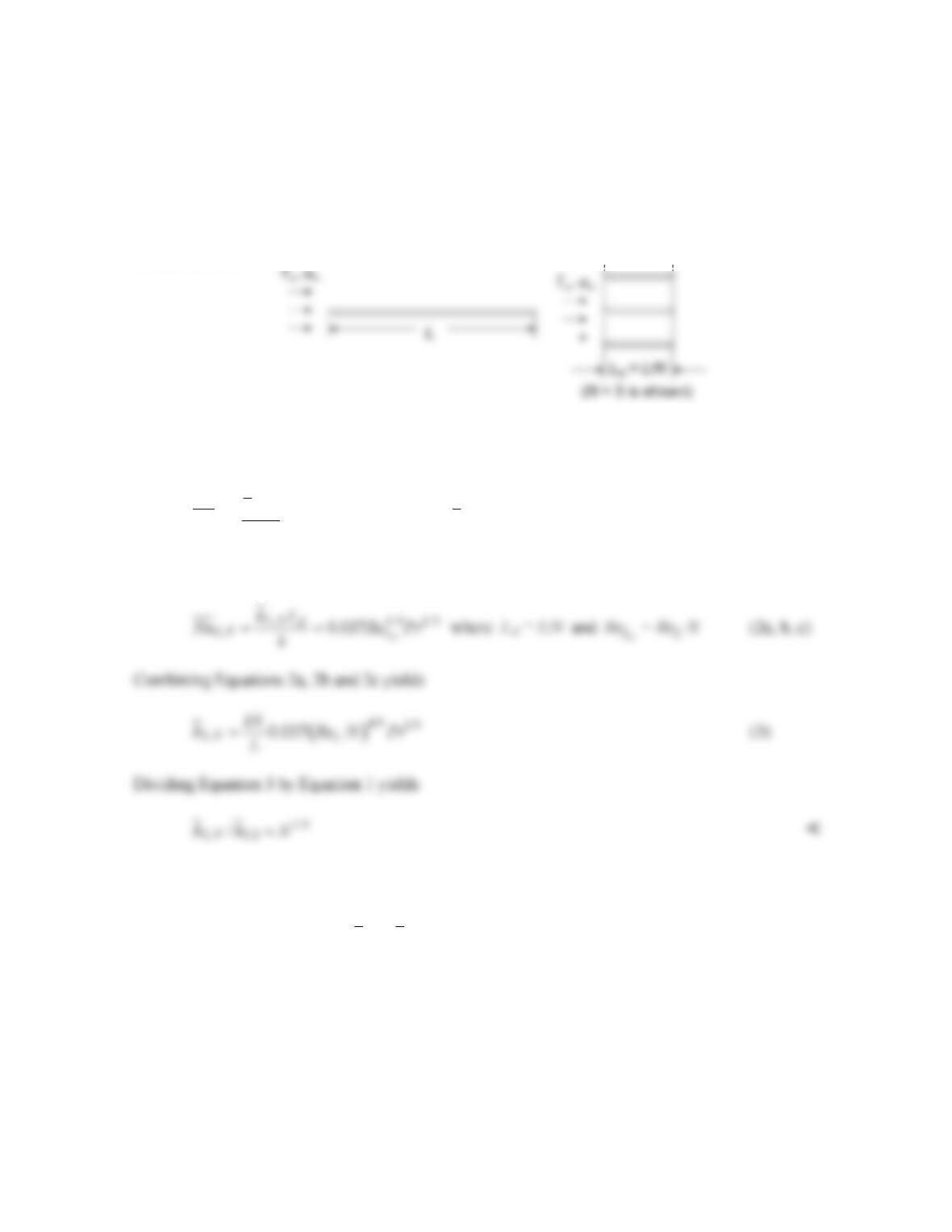
SCHEMATIC:
ASSUMPTIONS: (1) Laminar flow, (2) Constant properties.
ANALYSIS: For the single plate, Equation 7.30 applies
For the multiple plates,
Combining Equations 2a, 2b and 2c yields
Dividing Equation 3 by Equation 1 yields
COMMENTS: (1) By breaking the single plate into shorter segments, the average boundary layer
thickness is reduced, resulting in an increase of the average heat transfer coefficient. This is an
effective strategy for heat transfer enhancement. (2) If the boundary layer over the single plate is not
completely laminar, breaking it into shorter segments may or may not result in an increase in the
average heat transfer coefficient since the turbulent section of the boundary layer over the single plate
may be eliminated. (3) The relationship for completely turbulent flow is
1/5
/
N
LL
hhN=
, revealing
less sensitivity to the plate length than for laminar conditions.
PROBLEM 7.9
KNOWN: Length of isothermal flat plate in parallel flow, L.
FIND: Expression for the average heat transfer coefficients for N plates each of length LN = L/N to
the average heat transfer coefficient for the single plate.
SCHEMATIC:
ASSUMPTIONS: (1) Turbulent flow, (2) Constant properties.
ANALYSIS: Since Rex,c = 0, Equation 7.39 yields A = 0. Therefore, for the single plate,
,1 4/5 1/3
0.037
L
LL
hL
Nu Re Pr
k
= =
or
( )
4/5 1/3
,1 / 0.037
LL
h k L Re Pr=
(1)
For the multiple plates,
COMMENTS: (1) By breaking the single plate into shorter segments, the average boundary layer
thickness is reduced, resulting in a slight increase of the average heat transfer coefficient. Hence,
breaking the plate into shorter lengths results in modest heat transfer enhancement. (2) The
relationship for laminar flow is
1/2
,
/
LN L
h hN=
, revealing more sensitivity to the plate length for
laminar conditions.
PROBLEM 7.10
KNOWN: Dimensions and surface temperatures of a flat plate. Velocity and temperature of air
and water flow parallel to the plate.
FIND: (a) Average convective heat transfer coefficient, convective heat transfer rate, and drag
force when L = 2 m, w = 2 m. (b) Average convective heat transfer coefficient, convective heat
transfer rate, and drag force when L = 0.1 m, w = 0.1 m.
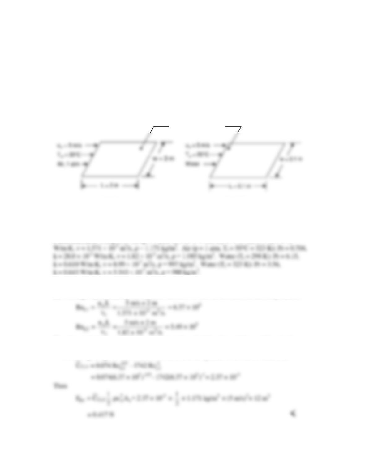
SCHEMATIC:
Ts= 50°C or 80°C
(a) Air (b) Water
Ts= 50°C or 80°C
(a) Air (b) Water
T
s
= 30°C or 80°C
ASSUMPTIONS: (1) Steady–state conditions, (2) Boundary layer assumptions are valid, (3)
Constant properties, (4) Transition Reynolds number is 5 × 10⁵.
PROPERTIES: Using IHT, Air (p = 1 atm, Tf = 25°C = 298 K): Pr = 0.708, k = 26.1 × 10⁻³
ANALYSIS:
(a) We begin by calculating the Reynolds numbers for the two different surface temperatures:
Therefore, in both cases the flow is turbulent at the end of the plate and the conditions in the
boundary layer are “mixed.”
The average drag coefficient can be calculated from Equation 7.40. For the first case,
Continued…
PROBLEM 7.10 (Cont.)
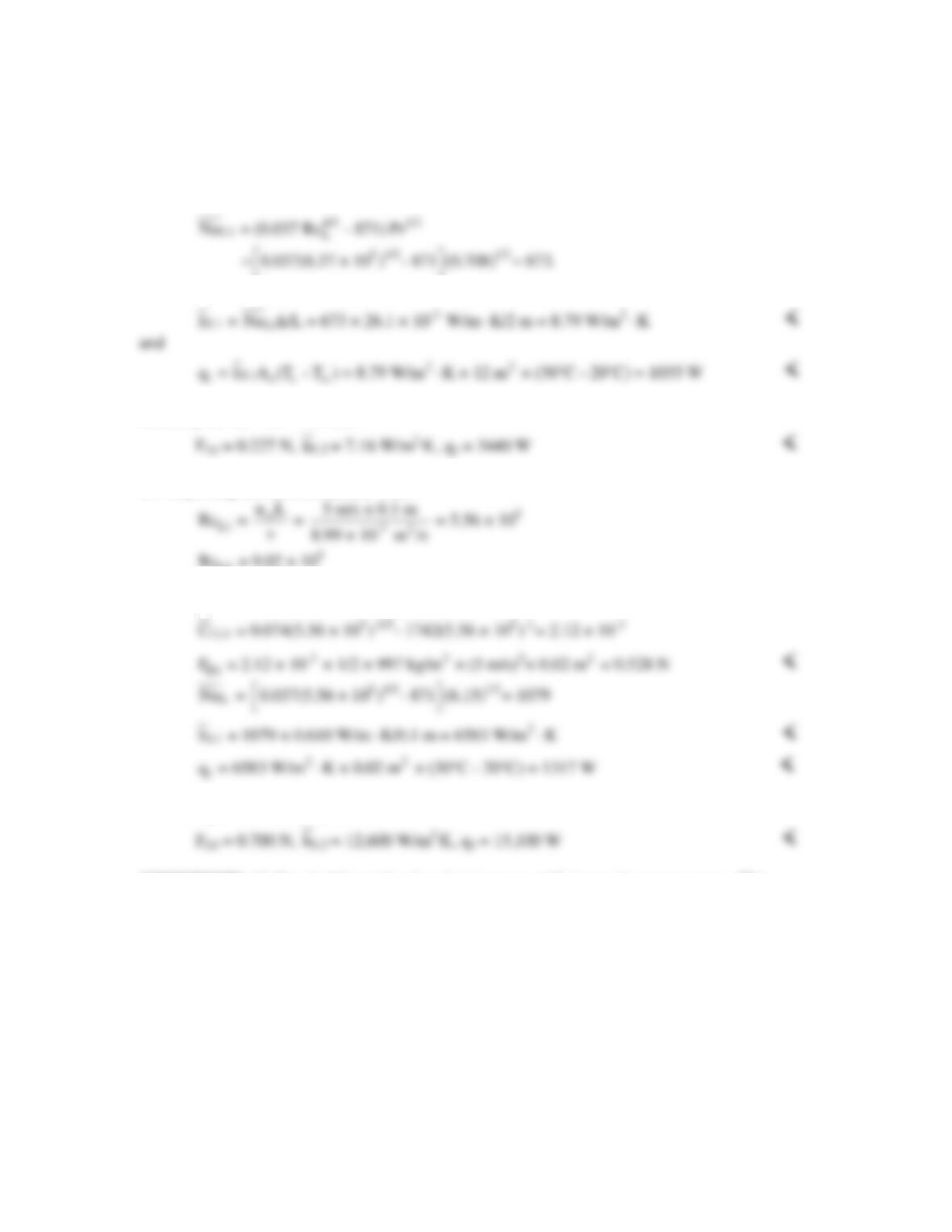
The average Nusselt number is calculated from Equation 7.38, with A = 871 for a transition
Reynolds number of 5 × 10⁵.
Then
Similarly for Ts = 80°C we find
(b) Repeating the calculations for water
L2
Re = 9.02 × 10
The flow is turbulent at the end of the plate in both cases.
For the higher surface temperature,
COMMENTS: (1) For air, kinematic viscosity increases with increasing temperature. This
decreases the Reynolds number which causes the transition to turbulence to move downstream,
thereby decreasing the drag force and average heat transfer coefficient. The heat transfer rate
increases for the higher surface temperature, however, because of the greater temperature
difference between the surface and air. (2) For water, kinematic viscosity decreases with
increasing temperature, causing the opposite trends as for air. The heat transfer rate increases
dramatically for the higher surface temperature because of the increases in both the heat transfer
coefficient and temperature difference. (3) Even though the water flows over a plate that is 600
times smaller, the drag force and heat transfer rate are larger than for air because of the smaller
viscosity and greater density, thermal conductivity, and Prandtl number. (4) The problem
highlights the importance of carefully accounting for the temperature dependence of thermal
properties.
PROBLEM 7.11
KNOWN: Freestream velocity and temperature of air in parallel flow over a flat plate. Plate temperature.
Critical Reynolds number for first case. Tripped to turbulence at x = 0 m in second case.
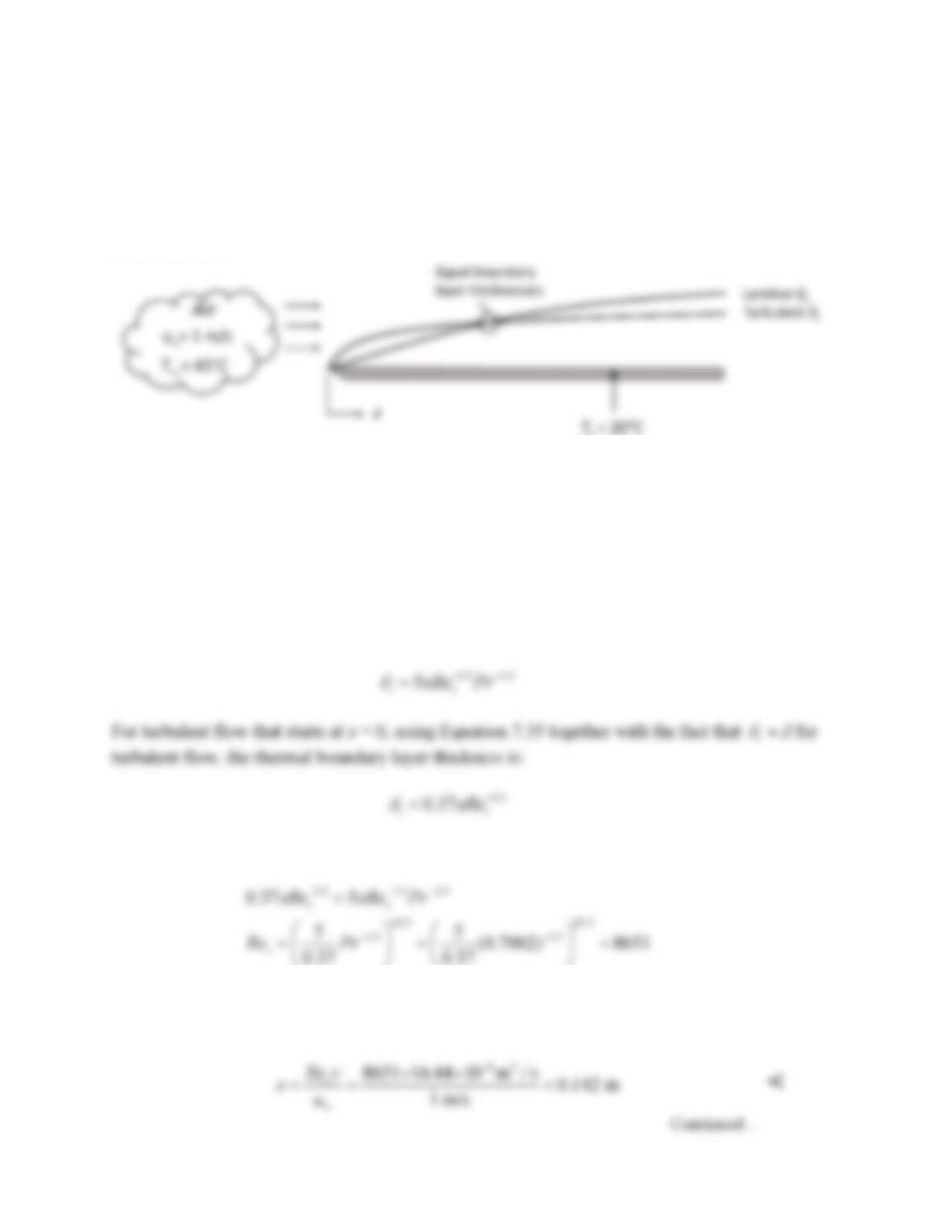
FIND: The x-location at which thermal boundary layer thicknesses are equal for the two cases. Local
heat fluxes at this location for the two cases.
SCHEMATIC:
ASSUMPTIONS: (1) Steady–state conditions, (2) Boundary layer assumptions are valid, (3) Constant
properties, (4) Transition Reynolds number is 5 × 10⁵ in Case 1, (5) For Case 2, a turbulent boundary
layer exists starting from x = 0.
PROPERTIES: Table A-4, Air, (T = 305.5 K): k = 0.02671 W/m⋅K,
ν
= 16.44 × 10⁻⁶ m2/s, Pr = 0.7062.
ANALYSIS: We begin by assuming that the case that is not tripped is still laminar at the x–location in
question. For laminar flow, taking Equations 7.19 and 7.24 together, the thermal boundary layer thickness
is:
Equating these two expressions and solving for x yields
Note that Rex < 5 × 10⁵, so the case that is not tripped to turbulence is indeed laminar at this
location as assumed. Then,
PROBLEM 7.11 (Cont.)
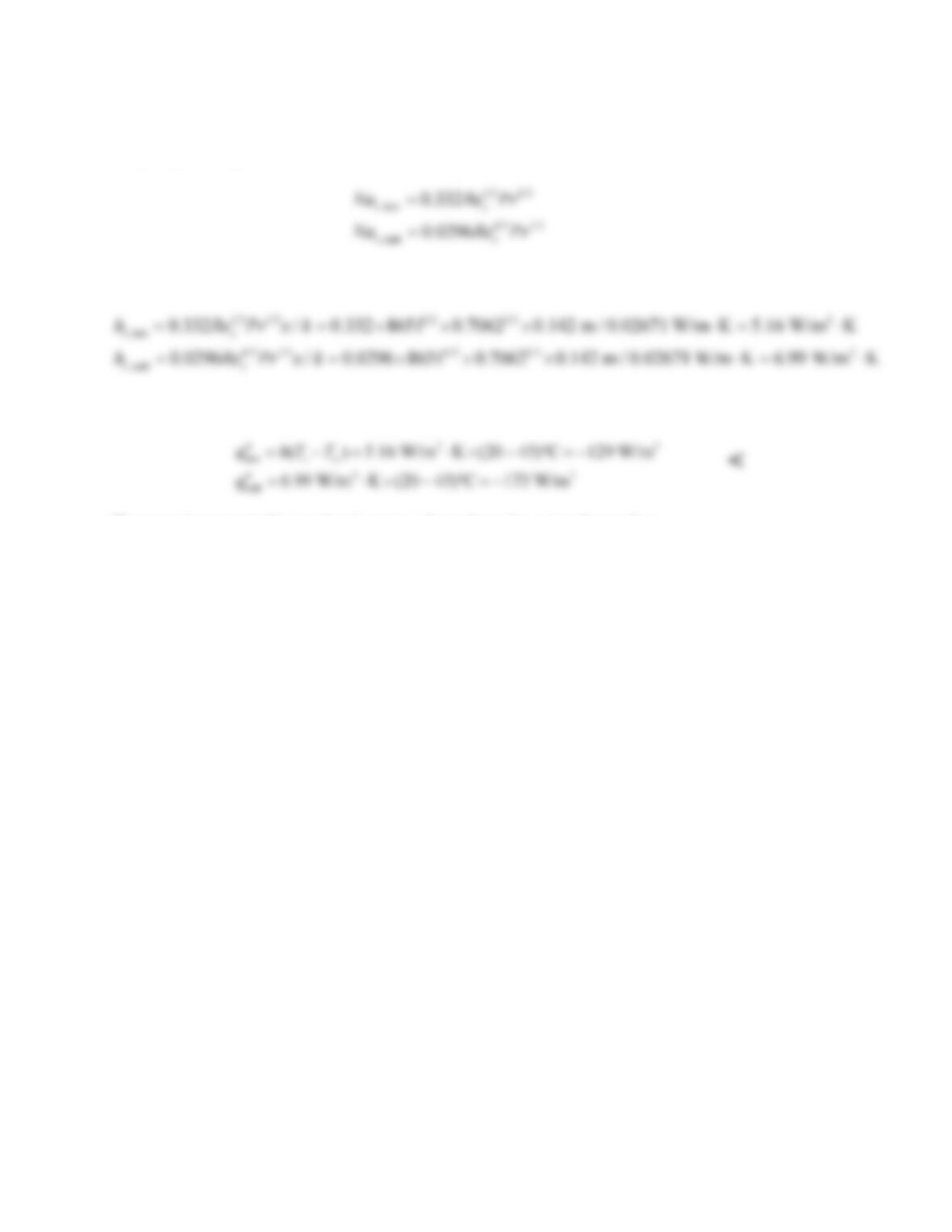
The local Nusselt numbers for the laminar and turbulent cases are given by Equations 7.23 and
7.36, respectively:
Therefore the local heat transfer coefficients are
And finally, the local heat fluxes are given by
The negative sign indicates that heat transfer is from the air to the surface.
COMMENTS: (1) If the air is not dry, condensation may occur, affecting the heat fluxes. (2) Note that
the heat flux is larger for the turbulent boundary layer due to the mixing that is an inherent feature of
turbulent flow.
PROBLEM 7.12
KNOWN: Freestream velocity and temperature of air in parallel flow over a flat plate. Plate temperature
and width. Length of segmented heaters on plate.
FIND: Which heater segment has minimum power requirement and what the power requirement is.
SCHEMATIC:
ASSUMPTIONS: (1) Steady–state incompressible flow conditions, (2) Boundary layer assumptions are
valid, (3) Constant properties, (4) Transition Reynolds number is 5 × 10⁵, (5) Negligible radiation effects,
(6) Bottom surfaces of heated segments are adiabatic, (7) There are six heater segments, for a total length
of L = 300 mm.
PROPERTIES: Table A-4, Air, (T = 483 K): k = 0.0395 W/m⋅K,
ν
= 36.61 × 10⁻⁶ m2/s, Pr = 0.685.
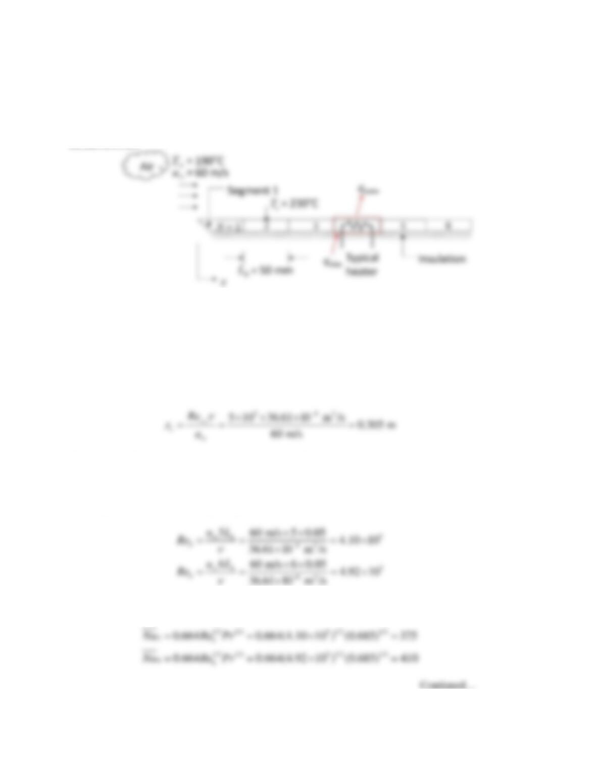
ANALYSIS: We begin by determining the location of transition to turbulence:
Therefore the flow is laminar everywhere. Since heat flux decreases as the boundary layer grows,
the minimum power requirement occurs on the sixth heater. <
The Reynolds numbers at the beginning and end of the sixth heater are:
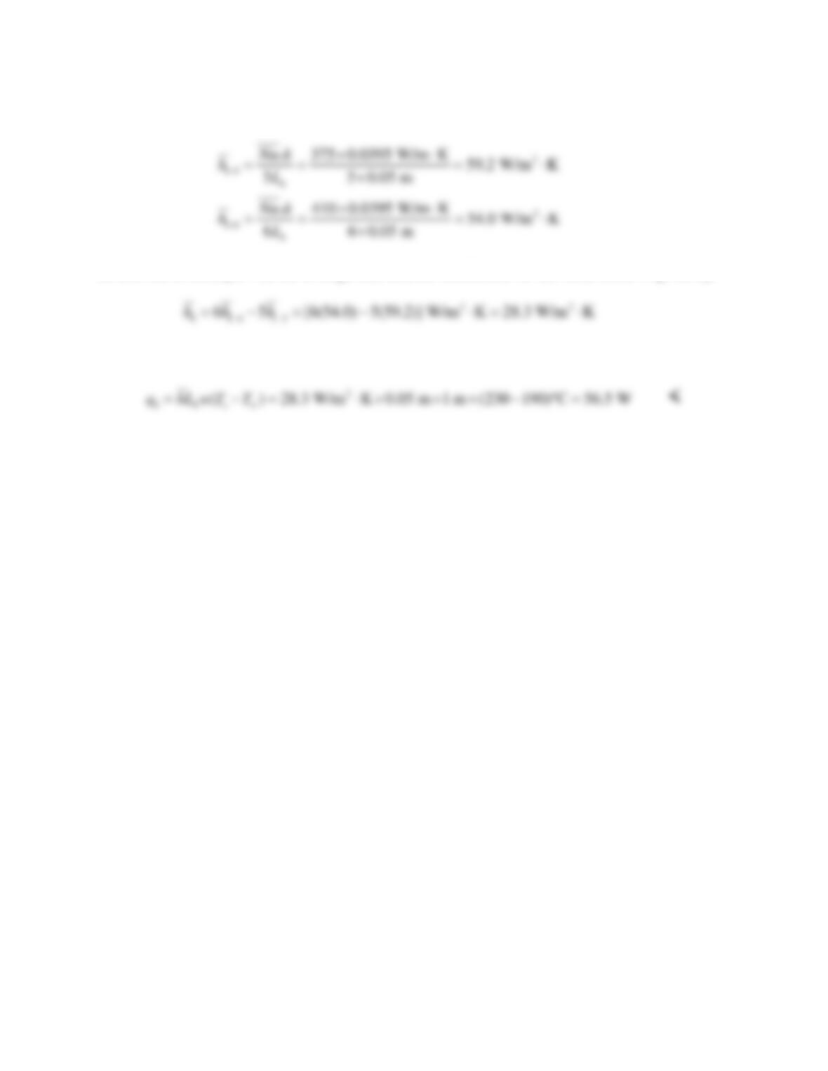
The average Nusselt numbers from x = 0 to the beginning and end of the sixth heater are:
PROBLEM 7.12 (Cont.)
The corresponding heat transfer coefficients are:
As derived in Example 7.2, the average heat transfer coefficient for the sixth heater is given by:
And the heater power is given by
COMMENTS: The higher freestream temperature in this problem as compared to Example 7.2 resulted
in a higher kinematic viscosity, which shifted the location of transition to turbulence further downstream.
PROBLEM 7.13
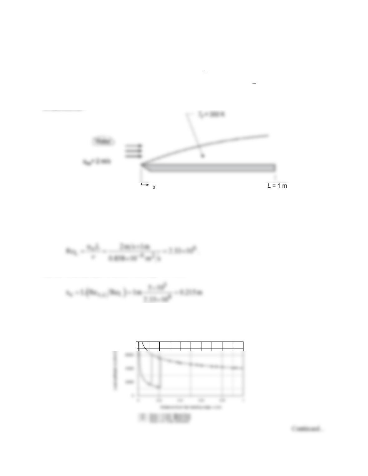
KNOWN: Velocity and temperature of water in parallel flow over a flat plate of 1-m length.
FIND: (a) Calculate and plot the variation of the local convection coefficient, hx (x), with distance for
flow conditions corresponding to transition Reynolds numbers of 5 × 10⁵, 3 × 10⁵ and 0 (fully turbulent),
(b) Plot the variation of the average convection coefficient,
( )
x
hx
, for the three flow conditions of part
(a), and (c) Determine the average convection coefficients for the entire plate,
h
L
, for the three flow
conditions of part (a).
SCHEMATIC:
ASSUMPTIONS: (1) Steady-state conditions, (2) Constant surface temperature, and (3) Critical
Reynolds depends upon prescribed flow conditions.
PROPERTIES: Table A.6, Water (300 K): ρ = 997 kg/m3, µ = 855 × 10-6 N⋅s/m2, ν = µ/ρ = 0.858 ×
10-6 m2/s, k = 0.613 W/m⋅K, Pr = 583.
ANALYSIS: (a) The Reynolds number for the plate (L = 1 m) is
and the boundary layer is mixed with Rex,c = 5 × 10⁵,
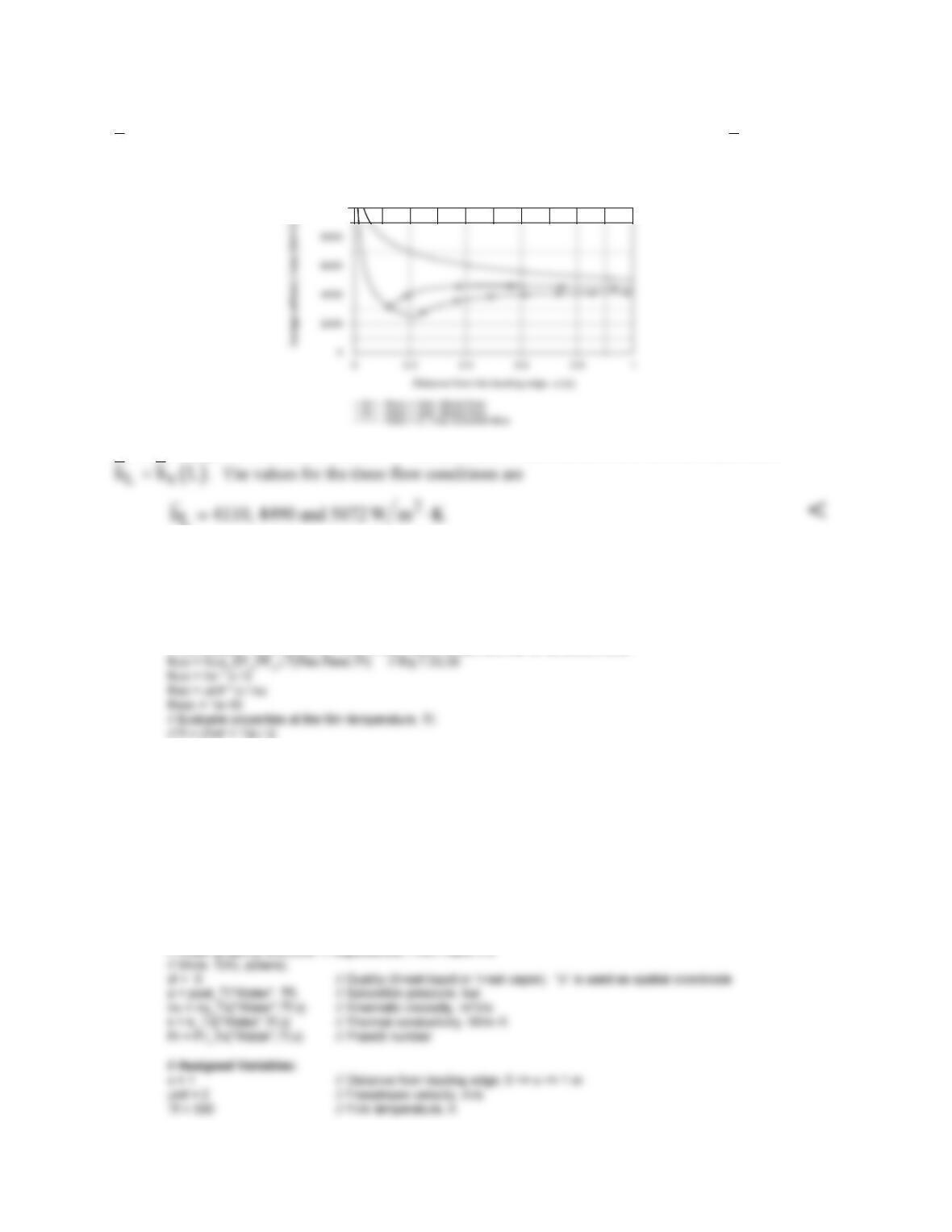
Using the IHT Correlation Tool, External Flow, Local coefficients for Laminar or Turbulent Flow, hx(x)
was evaluated and plotted with critical Reynolds numbers of 5 × 10⁵, 3.0 × 10⁵ and 0 (fully turbulent).
Note the location of the laminar–turbulent transition for the first two flow conditions.
8000
PROBLEM 7.13 (Cont.)
(b) Using the IHT Correlation Tool, External Flow, Average coefficient for Laminar or Mixed Flow,
( )
x
hx
was evaluated and plotted for the three flow conditions. Note that the change in
( )
x
hx
at the
critical length, xc, is rather gradual, compared to the abrupt change for the local coefficient, hx(x).
10000
(c) The average convection coefficients for the plate can be determined from the above plot since
COMMENTS: A copy of the IHT Workspace used to generate the above plot is shown below.
/* Method of Solution: Use the Correlation Tools, External Flow, Flat Plate, for (i) Local, laminar or turbulent
flow and (ii) Average, laminar or mixed flow, to evaluate the local and average convection coefficients as a
function of position on the plate. In each of these tools, the value of the critical Reynolds number, Rexc, can
be set corresponding to the special flow conditions. */
// Correlation Tool: External Flow, Plate Plate, Local, laminar or turbulent flow.
/* Correlation description: Parallel external flow (EF) over a flat plate (FP), local coefficient; laminar flow (L) for
Rex<Rexc, Eq 7.23; turbulent flow (T) for Rex>Rexc, Eq 7.36; 0.6<=Pr<=60. See Table 7.9. */
// Correlation Tool: External Flow, Plate Plate, Average, laminar or mixed flow.
NuLbar = NuL_bar_EF_FP_LM(Rex,Rexc,Pr) // Eq 7.30, 7.38, 7.39
NuLbar = hLbar * x / k // Changed variable from L to x
//ReL = uinf * x / nu
//Rexc = 5.0E5
/* Correlation description: Parallel external flow (EF) over a flat plate (FP), average coefficient; laminar (L) if
ReL<Rexc, Eq 7.30; mixed (M) if ReL>Rexc, Eq 7.38 and 7.39; 0.6<=Pr<=60. See Table 7.9. */
// Properties Tool – Water:
PROBLEM 7.14
KNOWN: Solar cell material dimensions and properties, solar–to–electrical conversion efficiency
dependence on silicon temperature, solar irradiation and location where the irradiation is
absorbed, air velocity and temperature.
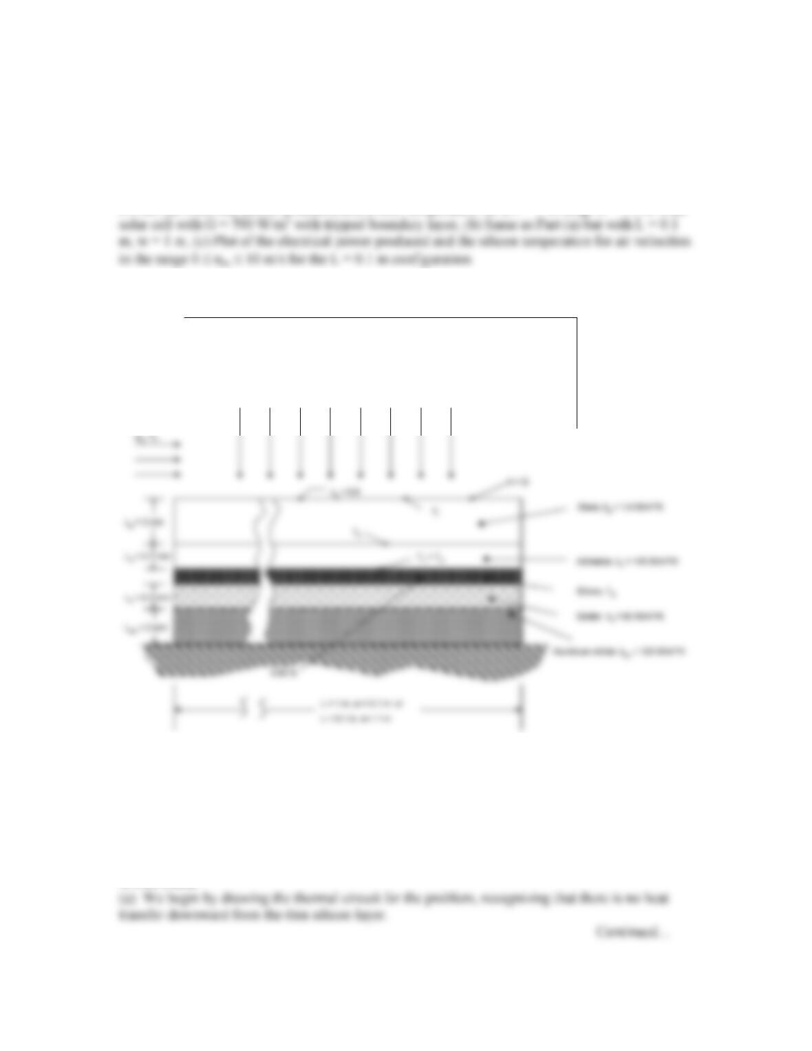
FIND: (a) Electrical power produced and silicon temperature for a L = 1 m long, w = 0.1 m wide
SCHEMATIC:
ASSUMPTIONS: (1) Steady-state conditions, (2) Constant properties, (3) One-dimensional heat
transfer, (4) Tripped and turbulent boundary layer, (5) Large surroundings, (6) Negligible contact
resistances.
PROPERTIES: Table A.4, air (assume Tf = 308 K, p = 1 atm): k = 0.0269 W/m⋅K, ν = 1.669 ×
10-5 m2/s, Pr = 0.706.
ANALYSIS:
G = 700 W/m
2
0 ≤u
m
≤ 10 m/s
T
sur
= 25°C
η= 0.28 –0.001°C
–1
(T
si
)
T
∞
= 25°C
G = 700 W/m
2
0 ≤u
m
≤ 10 m/s
T
sur
= 25°C
η= 0.28 –0.001°C
–1
(T
si
)
T
∞
= 25°C
20°C
20°C