Chapter 7
Chapter 7
Section 7.1
7.1.1If ~v is an eigenvector of A, then A~v =λ~v.
Hence A3~v =A2(A~v) = A2(λ~v) = A(Aλ~v) = A(λA~v) = A(λ2~v) = λ2A~v =λ3~v, so ~v is an eigenvector of A3with
eigenvalue λ3.
7.1.4We know A~v =λ~v, so 7A~v = 7λ~v, hence ~v is an eigenvector of 7Awith eigenvalue 7λ.
7.1.5Assume A~v =λ~v and B~v =β~v for some eigenvalues λ,β. Then (A+B)~v =A~v +B~v =λ~v +β~v = (λ+β)~v
so ~v is an eigenvector of A+Bwith eigenvalue λ+β.
7.1.9We want a b
c d 1
0=λ1
0for any λ. Hence a
c=λ
0, i.e., the desired matrices must have the form
λ b
0d, they must be upper triangular.
7.1.10 We want a b
c d 1
2= 5 1
2, i.e. the desired matrices must have the form 5−2b b
10 −2d d .
310
Section 7.1
7.1.14 We want to find all 4 ×4 matrices Asuch that A~e2=λ~e2, i.e. the second column of Amust be of the form
0
λ
0
0
, so A=
a0c d
e λ f g
h0i j
k0l m
.
7.1.15 Any vector on Lis unaffected by the reflection, so that a nonzero vector on Lis an eigenvector with eigenvalue
1. Any vector on L⊥is flipped about L, so that a nonzero vector on L⊥is an eigenvector with eigenvalue −1.
Picking a nonzero vector from Land one from L⊥, we obtain an eigenbasis. This transformation is diagonalizable.
7.1.19 Any nonzero vector in Lis an eigenvector with eigenvalue 1, and any nonzero vector in the plane L⊥is an
eigenvector with eigenvalue 0. Form an eigenbasis by picking any nonzero vector in Land any two nonparallel
vectors in L⊥. This transformation is diagonalizable.
7.1.20 Any nonzero vector along the ~e3-axis is unchanged, hence is an eigenvector with eigenvalue 1. No other (real)
eigenvalues can be found. There is no eigenbasis. This transformation fails to be diagonalizable.
7.1.21 Any nonzero vector in R3is an eigenvector with eigenvalue 5. Any basis for R3is an eigenbasis. This
transformation is diagonalizable.
311
Chapter 7
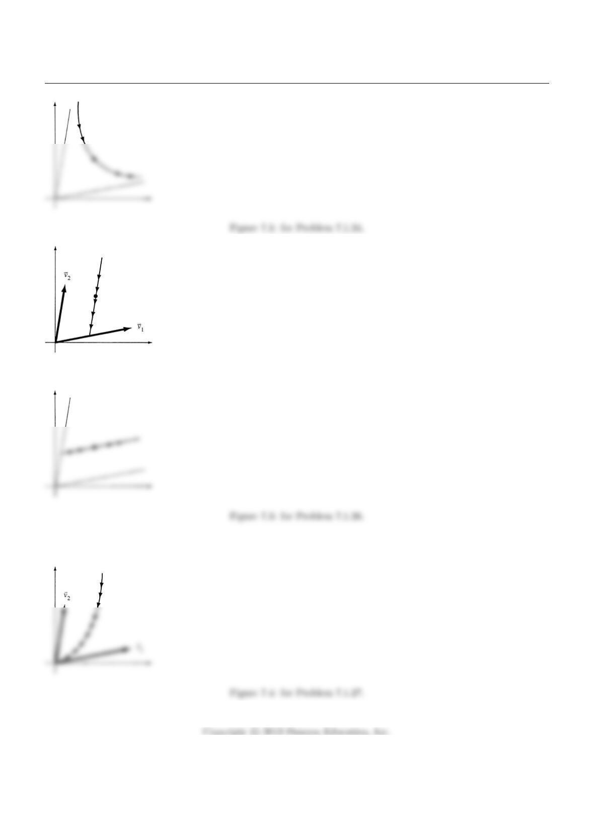
Figure 7.2: for Problem 7.1.25.
7.1.27 See Figure 7.4.
312
Section 7.1
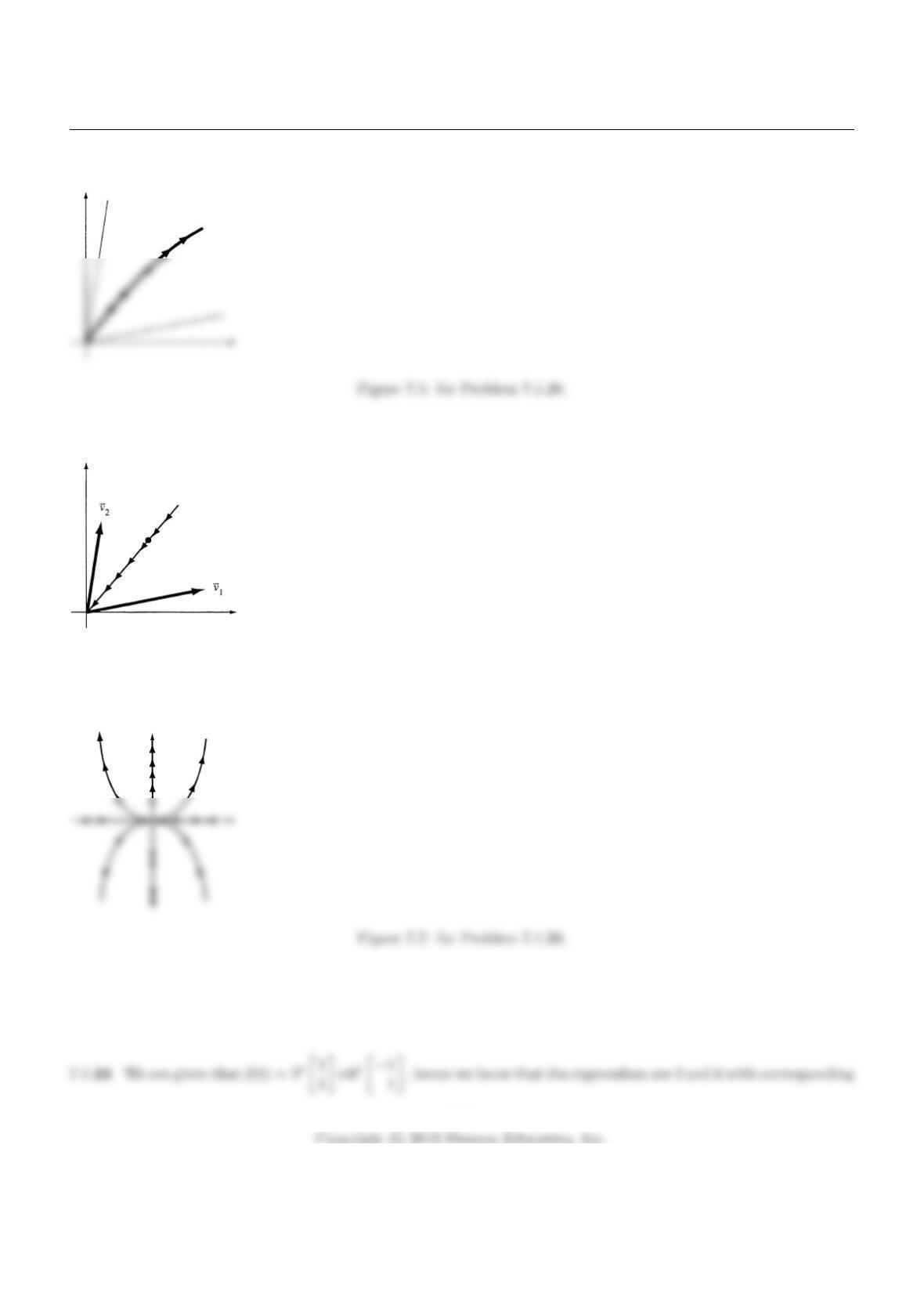
7.1.28 See Figure 7.5.
7.1.29 See Figure 7.6.
Figure 7.6: for Problem 7.1.29.
7.1.30 Since the matrix is diagonal, ~e1and ~e2are eigenvectors. See Figure 7.7.
7.1.31 See Figure 7.8.
7.1.32 Since the matrix is diagonal, ~e1and ~e2are eigenvectors. See Figure 7.9.
313
Chapter 7
eigenvectors 1
1and −1
1respectively (see Theorem 7.1.6), so we want a matrix Asuch that A1−1
1 1 =
2−6
2 6 . Multiplying on the right by 1−1
1 1 −1
, we get A=4−2
−2 4 .
7.1.34 (A2+ 2A+ 3In)~v =A2~v + 2A~v + 3In~v = 42~v + 2 ·4~v + 3~v = (16 + 8 + 3)~v = 27~v so ~v is an eigenvector of
A2+ 2A+ 3Inwith eigenvalue 27.
7.1.35 Let λbe an eigenvalue of S−1AS. Then for some nonzero vector ~v,S−1AS~v =λ~v, i.e., AS~v =Sλ~v =λS~v
α.
7.1.36 We want Asuch that A3
1=15
5and A1
2=10
20 , i.e. A3 1
1 2 =15 10
5 20 , so
Section 7.1
7.1.39 We want a b
c d 0
1=λ0
1=0
λ. So b= 0, and d=λ(for any λ). Thus, we need matrices of the form
a0
c d =a1 0
0 0 +c0 0
1 0 +d0 0
0 1 .
So, 1 0
0 0 ,0 0
1 0 ,0 0
0 1 is a basis of V, and dim(V)= 3.
7.1.41 We want a b
c d 1
1=λ11
1, and a b
c d 1
2=λ21
2. So, a+b=λ1=c+dand a+ 2b=λ2and
2λ2=c+ 2d.
7.1.42 We will do this in a slightly simpler manner than Exercise 40. Since A
1
0
0
is simply the first column of A,
the first column must be a multiple of ~e1. Similarly, the third column must be a multiple of ~e3. There are no
315
Chapter 7
5.
7.1.43 A=AIn=A[~e1. . . ~en] = [ λ1~e1. . . λn~en],where the eigenvalues λ1,…,λnare arbitrary. Thus A
can be any diagonal matrix, and dim(V) = n.
7.1.44 We see that each of the columns 1 through mof Awill have to be a multiple of its respective vector ~ei.
Thus, there will be mfree variables in the first mcolumns. The remaining n−mcolumns will each have nfree
variables. Thus, in total, the dimension of Vis m+ (n−m)n=m+n2−nm.
7.1.46 Since A~v = 3~v, we have ~v =1
3A~v =A1
3~v, so that ~v is in the image of A, as claimed.
7.1.49 For example, the matrix A=0 1
0 0 , with rank A= 1, fails to be diagonalizable. Since eigenvectors of A
must be in the image or in the kernel of A(by Exercise 47), the only eigenvectors of Aare of the form a
0,
where a6= 0 . Thus there is no eigenbasis for A.
7.1.51 We observe that rank A= 1 , and we will use the ideas presented in Exercises 47 and 48. Now ker A=
span −1
1and ImA= span 1
1, with A1
1=2
2= 2 1
1. Thus Ais diagonalizable, with S=
−1 1
1 1 and B=0 0
0 2 .
316
Section 7.1
7.1.53 We observe that rank A= 1 , and we will use the ideas presented in Exercises 47 and 48. Now ker A=
span
−2
1
0
,
−3
0
1
and ImA= span
1
2
3
, with A
1
2
3
= 14
1
2
3
. Thus Ais diagonalizable, with
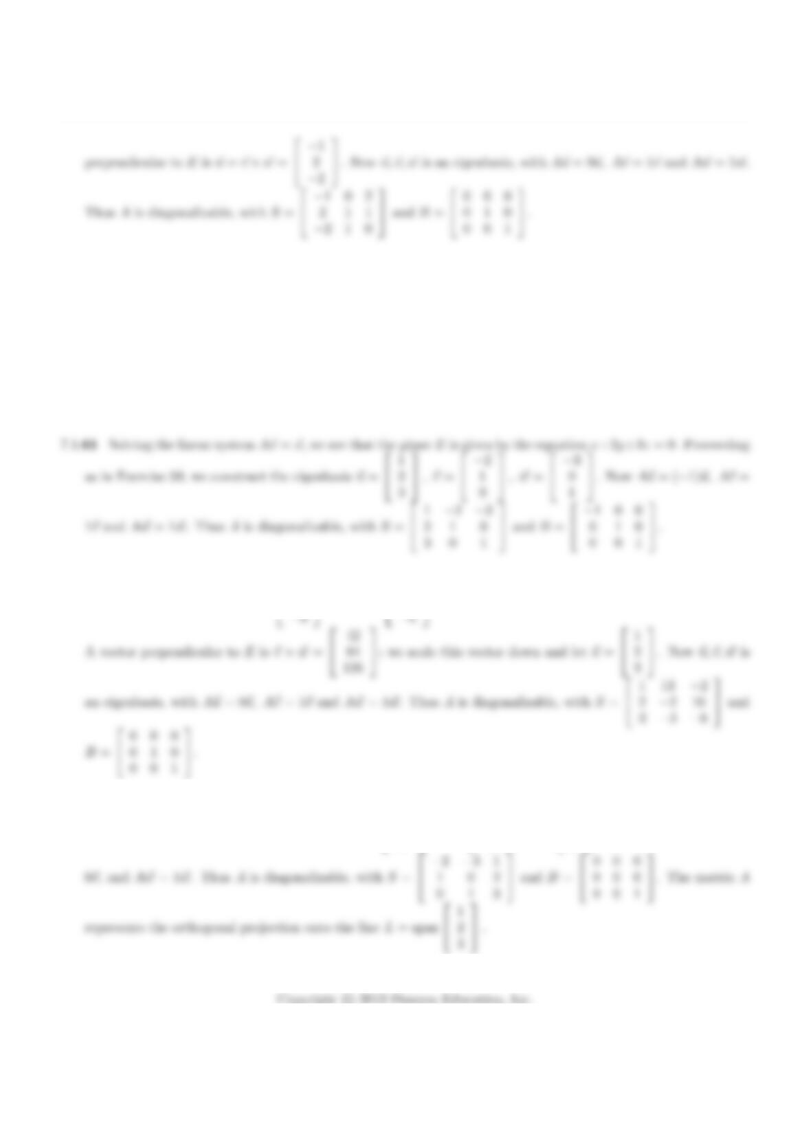
7.1.55 As in Example 3, we can pick a nonzero vector on L, for example, ~v =3
4, and a nonzero vector
perpendicular to L, for example, ~w =−4
3. Now ~v, ~w is an eigenbasis, with A~v =~v = 1~v and A ~w =~
0 = 0 ~w.
Thus Ais diagonalizable, with S=3−4
4 3 and B=1 0
0 0 .
7.1.57 Notice that the matrix Ais of the form A=a b
b−a, with a2+b2= 1, so that it represents the reflection
about a line L. Solving the equation A~x =~x, we find that L= span −3
1.To construct an eigenbasis ~v, ~w, we
can pick a nonzero vector on L, for example, ~v =−3
1, and a nonzero vector perpendicular to L, for example,
~w =1
3. NowA~v =~v = 1~v and A ~w =−~w = (−1) ~w. Thus Ais diagonalizable, with S=−3 1
1 3 and
B=1 0
0−1.
317
Chapter 7
7.1.60 Adapting the ideas developed in Example 3 and Exercise 59, we find the eigenbasis ~u =
−1
2
−2
, ~v =
0
1
1
, ~w =
2
1
0
, with A~u = (−1)~u, A~v = 1~v and A ~w = 1 ~w. Thus Ais diagonalizable, with S=
−1 0 2
2 1 1
−2 1 0
and B=
−1 0 0
0 1 0
0 0 1
.
7.1.62 A basis of E= ImAis ~v =
13
−2
and ~w =
−2
10
, corresponding to the first two columns of matrix A.
7.1.63 As in Exercise 53, we find the eigenbasis ~u =
−2
1
0
, ~v =
−3
0
1
, ~w =
1
2
3
. We have A~u = 0~u, A~v =
318
Section 7.1
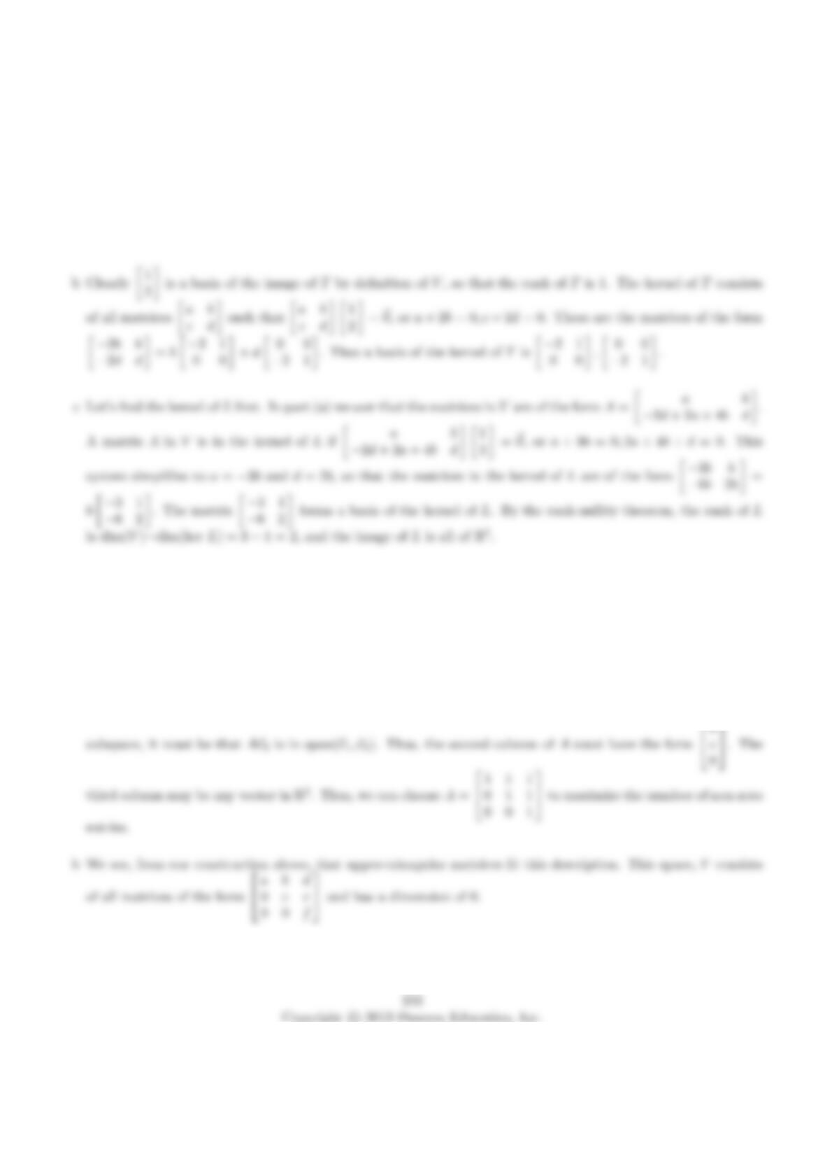
7.1.64 a We need all matrices Asuch that a b
c d 1
2=k1
2=k
2k.
Thus, a+ 2b=kand c+ 2d= 2k. So, c+ 2d= 2a+ 4b, or c=−2d+ 2a+ 4band Amust be of the form
a b
−2d+ 2a+ 4b d =a1 0
2 0 +b0 1
4 0 +d0 0
−2 1 . So a basis of Vis 1 0
2 0 ,0 1
4 0 ,0 0
−2 1 ,and
the dimension of Vis 3.
7.1.65 Suppose Vis a one-dimensional A-invariant subspace of Rn,and ~v is a non-zero vector in V. Then A~v will
be in V, so that A~v =λ~v for some λ, and ~v is an eigenvector of A. Conversely, if ~v is any eigenvector of A, then
V= span(~v) will be a one-dimensional A-invariant subspace. Thus the one-dimensional A-invariant subspaces V
are of the form V= span(~v),where ~v is an eigenvector of A.
7.1.66 a Since span(~e1) is an A-invariant subspace of R3,it must be that ~e1is an eigenvector of A, as revealed in
Exercise 65. Thus, the first column of Amust be of the form
a
0
0
. Since span(~e1, ~e2) is also an A-invariant
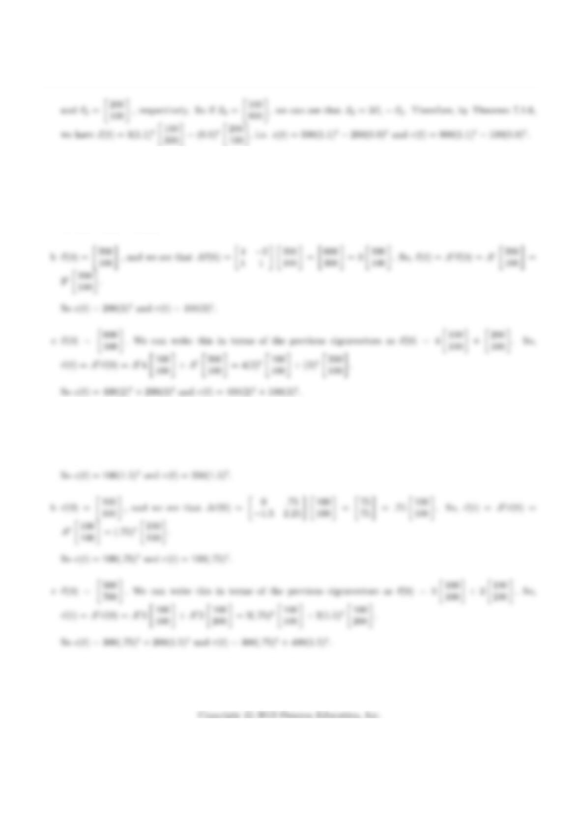
7.1.67 The eigenvalues of the system are λ1= 1.1, and λ2= 0.9 and corresponding eigenvectors are ~v1=100
300
Chapter 7
7.1.68 a~v(0) = 100
100 ,and we see that A~v(0) = 4−2
1 1 100
100 =200
200 = 2 100
100 . So, ~v(t) = At~v(0) =
At100
100 = 2t100
100 .
So c(t) = r(t) = 100(2)t.
7.1.69 a~v(0) = 100
200 ,and we see that A~v(0) = 0.75
−1.5 2.25 100
200 =150
300 = 1.5100
200 . So, ~v(t) = At~v(0) =
At100
200 = (1.5)t100
200 .
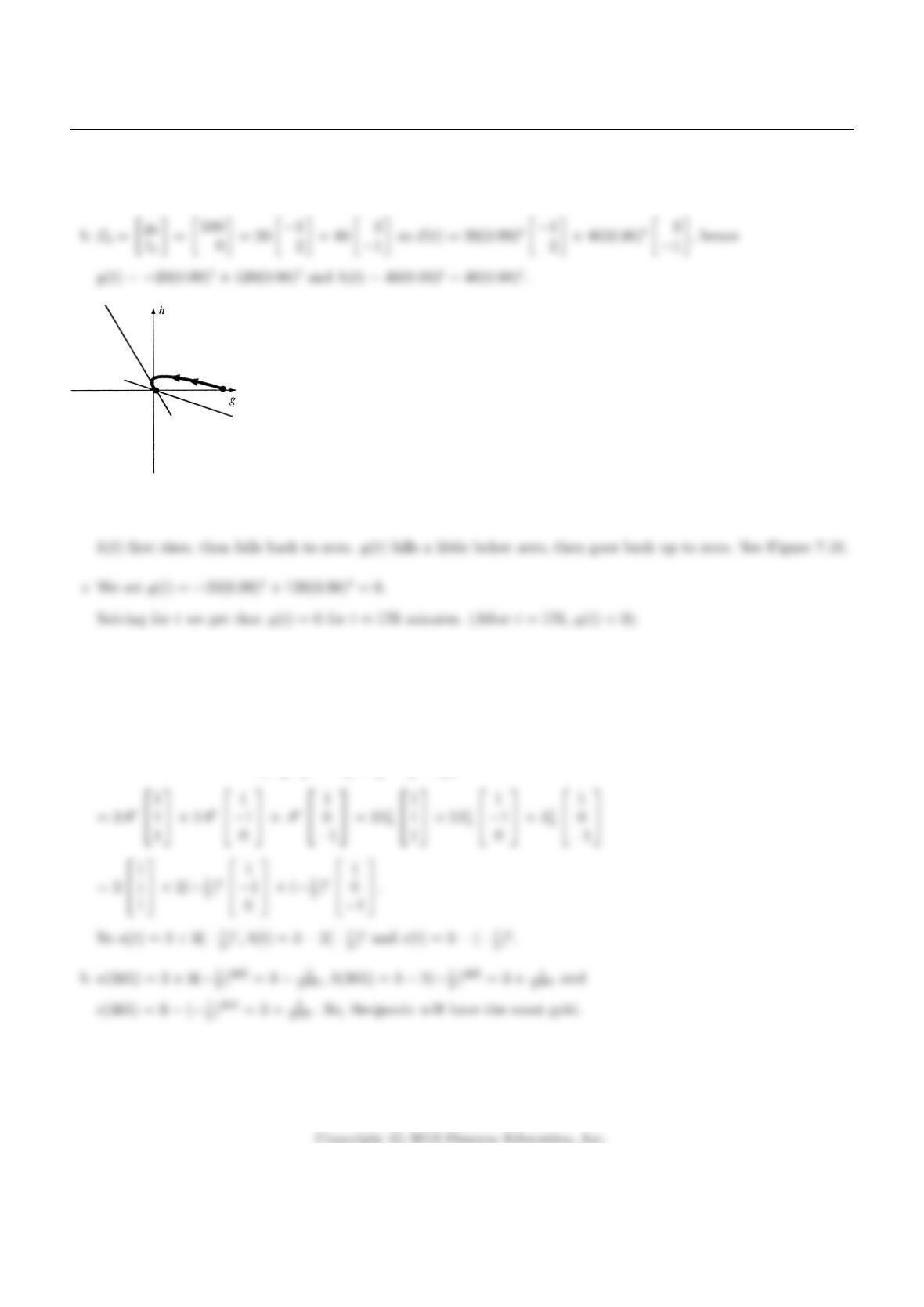
7.1.70 a0.978 −0.006
0.004 0.992 −1
2=−0.99
1.98 = 0.99 −1
2,
320
Section 7.1
and 0.978 −0.006
0.004 0.992 3
−1=2.94
−0.98 = 0.98 3
−1. The eigenvalues are λ1= 0.99 and λ2= 0.98.
Figure 7.10: for Problem 7.1.70b.
7.1.71 a~v(0) =
6
1
2
= 3
1
1
1
+ 2
1
−1
0
+
1
0
−1
.
So, ~v(t) = At~v(0) = At
3
1
1
1
+ 2
1
−1
0
+
1
0
−1
7.1.72 a We are given that
n(t+ 1) = 2a(t)
321
Chapter 7
Section 7.2
7.2.1λ1= 1, λ2= 3 by Theorem 7.2.2.
7.2.4det(A−λI2) = det −λ4
−1 4 −λ=−λ(4 −λ) + 4 = (λ−2)2= 0 so λ= 2 with algebraic multiplicity 2.
7.2.7λ= 1 with algebraic multiplicity 3, by Theorem 7.2.2.
7.2.8fA(λ) = −λ2(λ+ 3) so
322
Section 7.2
7.2.10 fA(λ) = (1 + λ)2(1 −λ) so λ1=−1 (Algebraic multiplicity 2), λ2= 1.
7.2.14 fA(λ) = det(B−λI2) det(D−λI2) (see Theorem 6.1.5).
The eigenvalues of Aare the eigenvalues of Band D. The eigenvalues of Care irrelevant.
7.2.15 fA(λ) = λ2−2λ+ (1 −k) = 0 if λ1,2=2±√4−4(1−k)
2= 1 ±√k
The matrix Ahas 2 distinct real eigenvalues when k > 0, no real eigenvalues when k < 0.
7.2.19 True, since fA(λ) = λ2−tr(A)λ+ det(A) and the discriminant [tr(A)]2−4 det(A) is positive if det(A) is
negative.
7.2.20 If ~v1and ~v2are eigenvectors with eigenvalues λ1and λ2, respectively, then ~v1, ~v2will be an eigenbasis, so
that matrix Ais diagonalizable as claimed.
323
Chapter 7
7.2.24 λ1= 0.25, λ2= 1
7.2.25 Ab
c=ab +cb
cb +cd =(a+c)b
(b+d)c=b
csince a+c=b+d= 1; therefore, b
cis an eigenvector with
7.2.26 Here b
c=0.25
0.5with λ1= 1 and 1
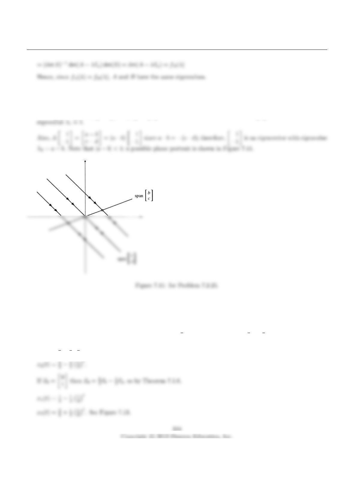
−1with λ2=a−b= 0.25. See Figure 7.12.
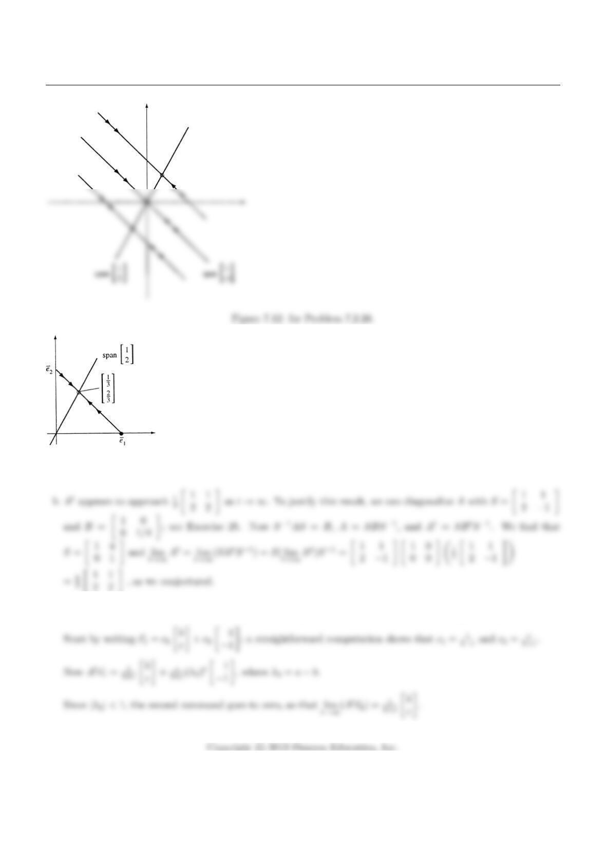
7.2.27 a We know ~v1=1
2, λ1= 1 and ~v2=1
−1, λ2=1
4. If ~x0=1
0then ~x0=1
3~v1+2
3~v2, so by Theorem 7.1.6,
x1(t) = 1
3+2
31
4t
Section 7.2
Figure 7.13: for Problem 7.2.27a.
c Let us think about the first column of At, which is At~e1. We can use Theorem 7.1.6 to compute At~e1.
325
Chapter 7
b The eigenvectors of Aare 0.1
0.2or 1
2with λ1= 1, and 1
−1with λ2= 0.7.
~x0=1200
0= 400 1
2+ 800 1
−1so ~x(t) = 400 1
2+ 800(0.7)t1
−1or
7.2.29 The ith entry of A~e is [ai1ai2···ain]~e =
n
X
j=1
aij = 1, so A~e =~e and λ= 1 is an eigenvalue of A, corresponding
to the eigenvector ~e.
7.2.30 a Suppose A~v =λ~v. Let vibe the largest component of ~v, meaning that vi≥vjfor all j= 1, …, n. Then the
ith component of A~v is
326
Section 7.2
It follows that |λ| ≤ 1, as claimed.
c. In part b, we see that |λ|= 1 if (and only if) both of the equations
Pn
=Pn
7.2.31 Since Aand AThave the same eigenvalues (by Exercise 22), Exercise 29 states that λ= 1 is an eigenvalue
of A, and Exercise 30 says that |λ| ≤ 1 for all eigenvalues λ. Vector ~e need not be an eigenvector of A; consider
A=0.9 0.9
0.1 0.1.
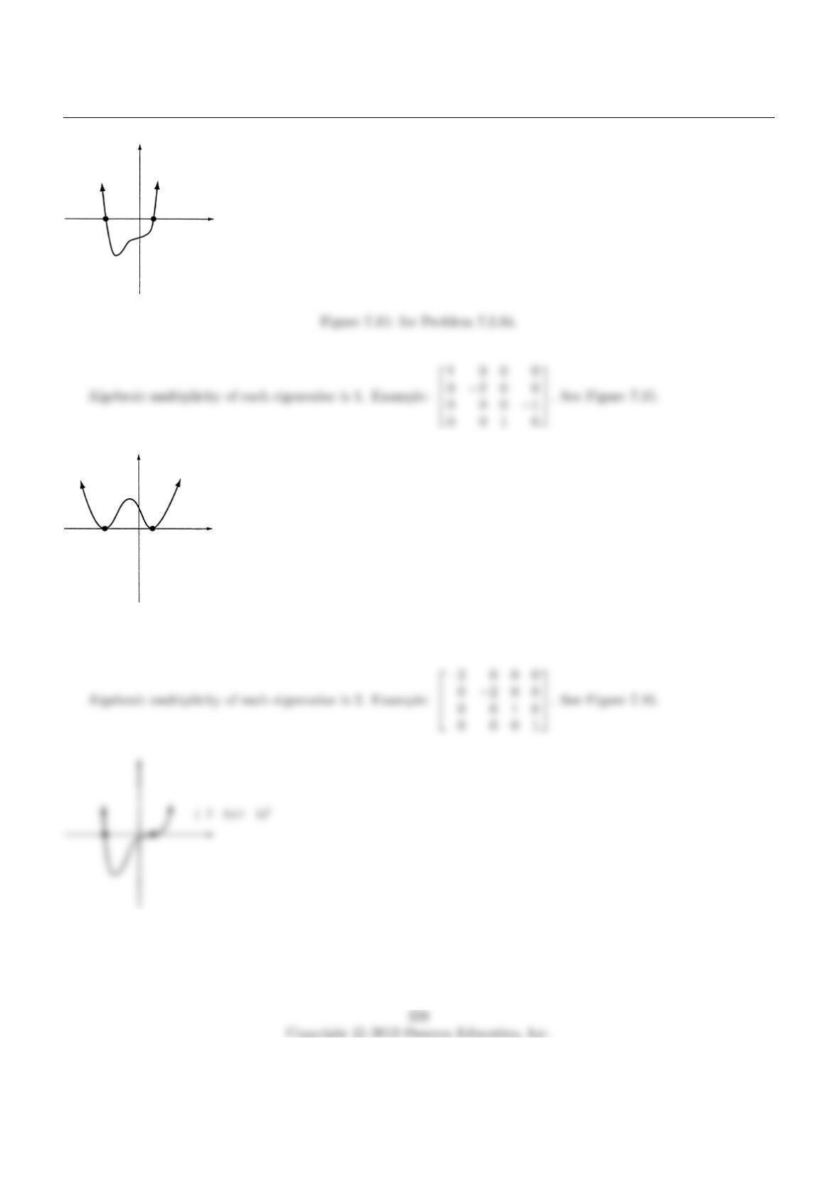
7.2.32 fA(λ) = −λ3+ 3λ+k. The eigenvalues of Aare the solutions of the equation −λ3+ 3λ+k= 0,or,
λ3−3λ=k. Following the hint, we graph the function g(λ) = λ3−3λas shown in Figure 7.14. We use the
derivative f′(λ) = 3λ2−3 to see that g(λ) has a global minimum at (1,−2) and a global maximum at (−1,2).
Figure 7.14: for Problem 7.2.32.
7.2.33 afA(λ) = det(A−λI3) = −λ3+cλ2+bλ +a
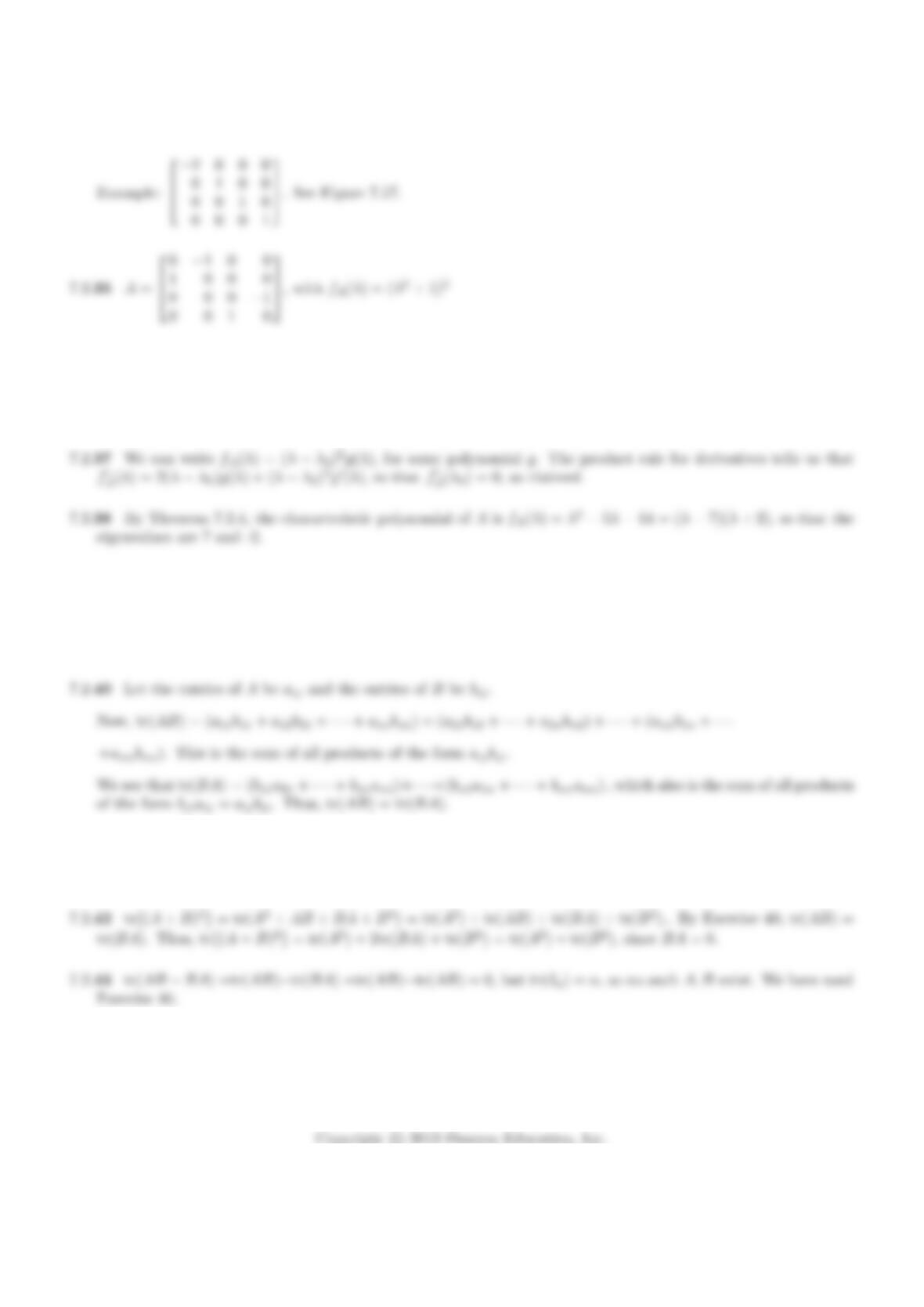
7.2.34 Consider the possible graphs of fA(λ) assuming that it has 2 distinct real roots.
327
Chapter 7
(1 – λ) (–2 – λ) (λ2 + 1)
(–2 – λ)2 (1 – λ)2
Figure 7.16: for Problem 7.2.34.
Figure 7.17: for Problem 7.2.34.
Algebraic multiplicity of λ1is 1, and of λ2is 3.
Section 7.2
7.2.36 Let A=
B0
B...
0B
where B=0−1
1 0 , fA(λ) = (λ2+ 1)n.
7.2.39 tr(AB) =tra b
c d e f
g h =trae +bg −−−
−−− cf +dh =ae +bg +cf +dh.
tr(BA) =tre f
g h a b
c d =trea +fc −−−
−−− gb +hd =ea +fc +gb +hd. So they are equal.
7.2.41 So there exists an invertible Ssuch that B=S−1AS, and tr(B) =tr(S−1AS)
=tr((S−1A)S). By Exercise 40, this equals tr(S(S−1A)) =tr(A).
7.2.44 No, there are no such matrices Aand B. We will argue indirectly, assuming that invertible matrices Aand
Bwith AB −BA =Ado exist. Then AB =BA +A= (B+In)A, and ABA−1=B+In. Using Exercise 41,
we see that tr(B) = tr(ABA−1) = tr(B+In) = tr(B) + n, a contradiction.
329