
PROBLEM 7.46 (Cont.)
Therefore, the heat transfer rate from the cylinder is,
COMMENTS: (1) The heat transfer coefficient associated with the cylinder is 80% greater than that
associated with the flat plate. However, for the same volume, the exposed surface area of the cylinder
PROBLEM 7.47
KNOWN: Temperature sensor of 10.5 mm diameter experiences cross–flow of water at 80°C and
velocity, 0.005 < V < 0.20 m/s. Sensor temperature may vary over the range 20 < Ts < 80°C.
FIND: Expression for convection heat transfer coefficient as a function of Ts and V.
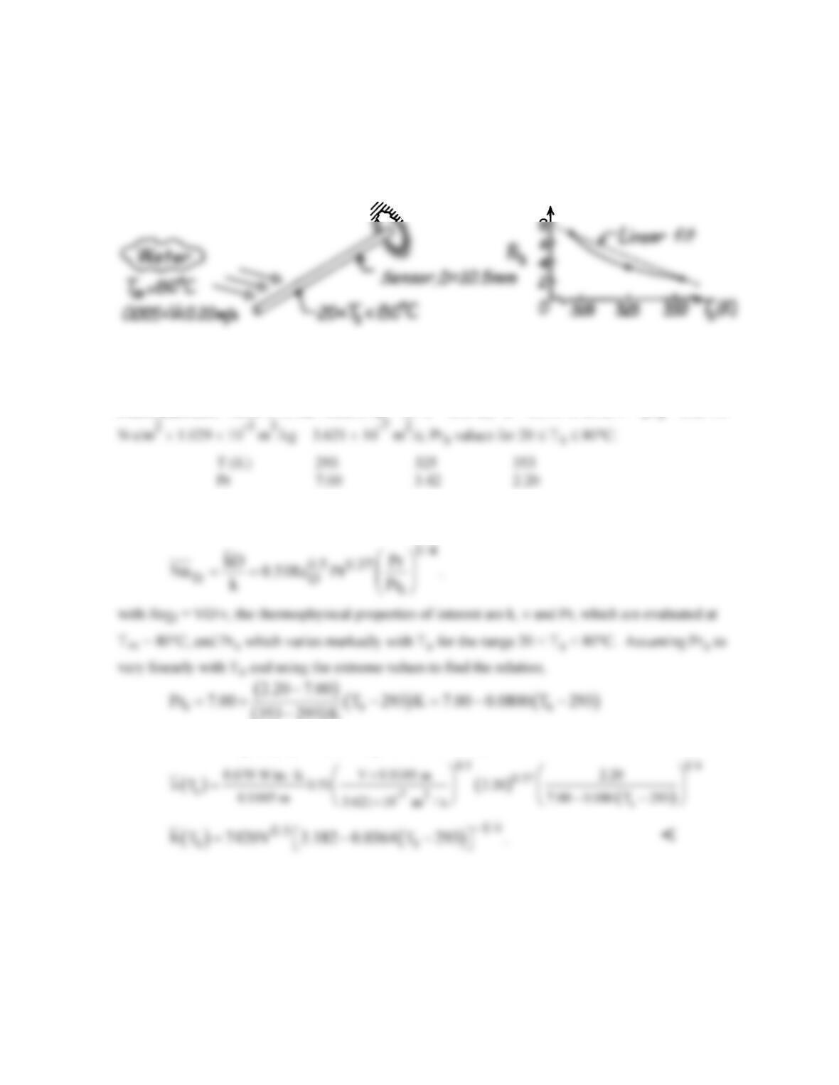
SCHEMATIC:
ASSUMPTIONS: (1) Steady-state conditions, (2) Sensor-water flow approximates a cylinder in
cross–flow, (3) Prandtl number varies linearly with temperature over the range of interest.
PROPERTIES: Table A-6, Sat. water (T∞ = 80°C = 353 K): k = 0.670 W/m⋅K, ν = µvf = 352×10-6
ANALYSIS: Using the Zukauskus correlation for the range 40 < ReD < 4000 with C = 0.51 and m =
0.5,
( ) ( ) ( )
where the units of Ts are [K]. Substituting numerical values, find
COMMENTS: (1) From the Prs vs. Ts graph above, a linear fit is seen to be poor for this
temperature range. However, because the Prs dependence is to the ¼ power, the discrepancy may be
acceptable. (2) The minimum and maximum Reynolds numbers are 145 and 5800, respectively. Hence
the usage of the Zukauskas constants in this solution are appropriate.
PROBLEM 7.48
KNOWN: Aluminum transmission line with a diameter of 20 mm having an electrical resistance of
R′
= 2.636×10⁻⁴ ohm/m carrying a current of 700 A subjected to severe cross winds. To reduce
potential fire hazard when adjacent lines make contact and spark, insulation is to be applied.
FIND: (a) The bare conductor temperature when the air temperature is 20°C and the line is subjected
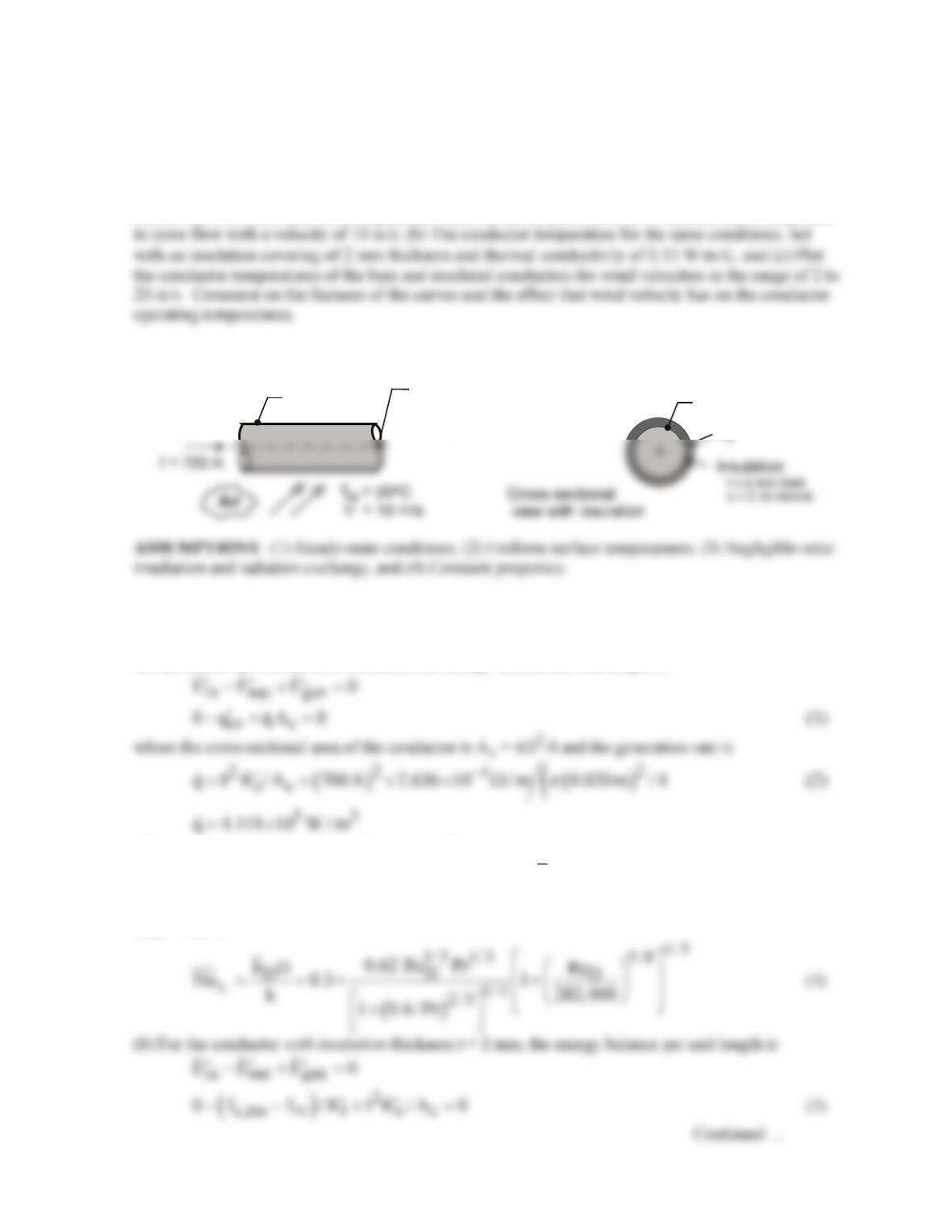
SCHEMATIC:
Conductor (bare)
D = 20 mm
= 2.636×10– Rm
e4
Ω
/
‘
Tc,bare Tc,ins
Ts
PROPERTIES: Table A-4, Air (Tf = (Ts + T∞)/2, 1 atm): evaluated using the IHT Properties
library with a Correlation function; see Comment 2.
ANALYSIS: (a) For the bare conductor the energy balance per unit length is
The convection rate equation can be expressed as
( )
( )
cv c,bare t t D
q T T / R R 1/ h D
π
∞
′ ′′
=−=×
(3,4)
and the convection coefficient is estimated using the Churchill-Bernstein correlation, Eq. 7.54, with
ReD = VD/ν,
PROBLEM 7.48 (Cont.)
where
t
R′
is the sum of the insulation conduction and convection process thermal resistances,
( ) ( ) ( )
t D 2t
R n D 2t / D / 2 k 1/ h D 2t
+
′
=+ ++
ππ
(6)
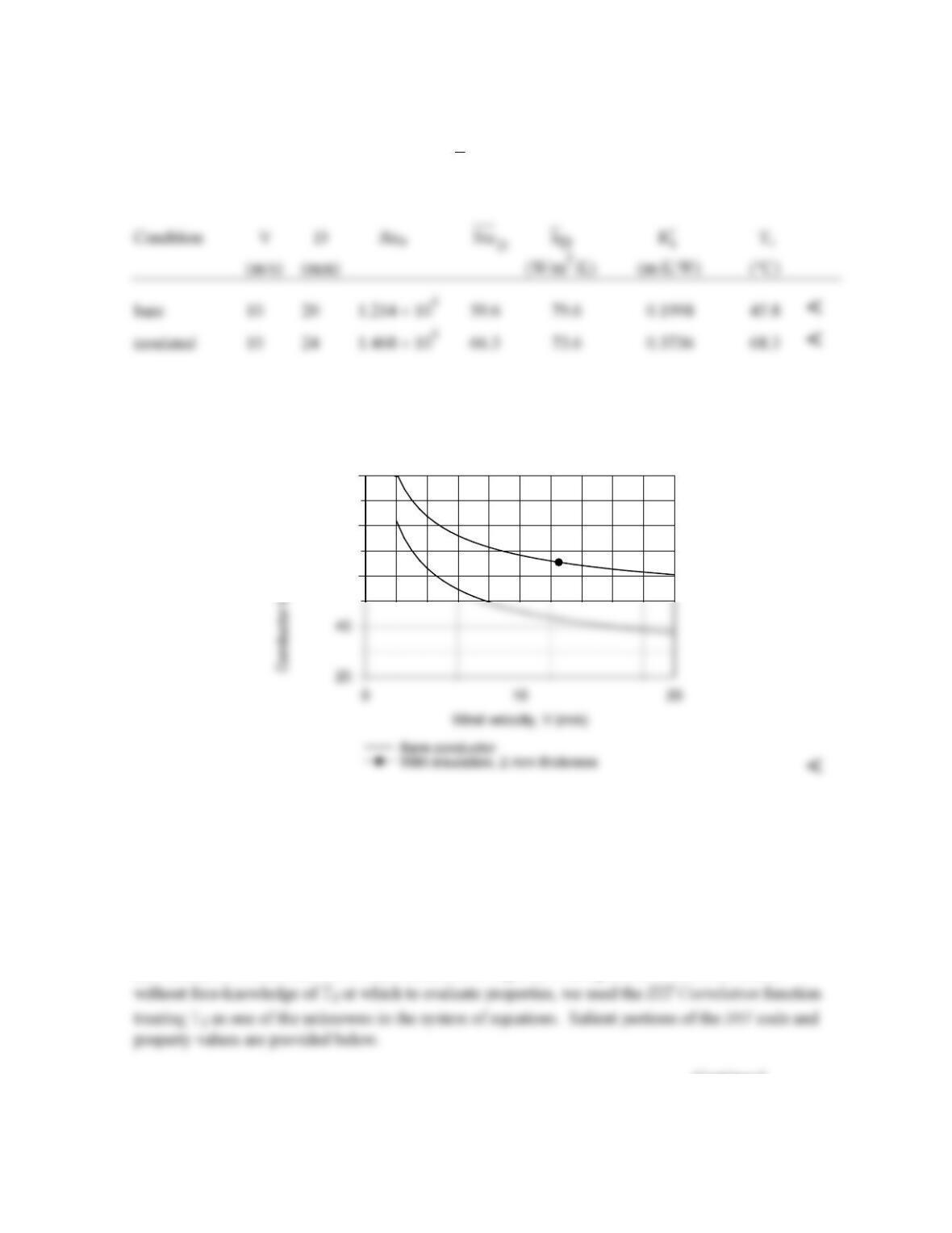
The results of the analysis using IHT are tabulated below.
(c) Using the IHT code with the foregoing relations, the conductor temperatures Tc,base and Tc,ins for
the bare and insulated conditions are calculated and plotted for the wind velocity range of 2 to 20 m/s.
60
80
100
COMMENTS: (1) The effect of the 2-mm thickness insulation is to increase the conductor operating
temperature by (68.3 – 46.1)°C = 22°C. While we didn’t account for an increase in the electrical
resistivity with increasing temperature, the adverse effect is to increase the I2R loss, which represents
a loss of revenue to the power provider. From the graph, note that the conductor temperature increases
markedly with decreasing wind velocity, and the effect of insulation is still around +20°C.
(2) Because of the tediousness of hand calculations required in using the convection correlation
Continued …
t
R′

PROBLEM 7.48 (Cont.)
// Forced convection, cross flow, cylinder
NuDbar = NuD_bar_EF_CY(ReD,Pr) // Eq 7.54
NuDbar = hDbar * Do / k
ReD = V * Do / nu // Outer diameter; bare or with insulation
(3) Is the temperature gradient within the conductor significant?
PROBLEM 7.49
KNOWN: Velocities and temperatures of two air streams separated by a wall. Dimensions of an
aluminum pin fin inserted through the wall. Distance it extends into the upper fluid.
FIND: (a) Heat transfer rate between the fluids via the pin fin, when it extends 50 mm into the upper
fluid. (b) Heat transfer rate as a function of the distance it extends into the upper fluid.
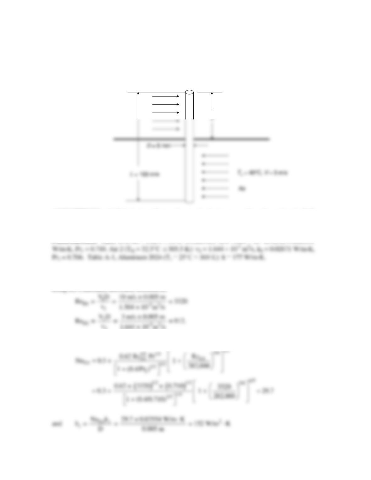
SCHEMATIC:
ASSUMPTIONS: (1) Velocity is uniform – decreased velocity near wall can be neglected, (2) For
the purpose of evaluating properties, the fin temperature is equal to the average of the two fluid
temperatures, Ts = 25°C.
PROPERTIES: Table A–4, Air 1 (Tf1 = 17.5°C
≅
290.5 K): ν1 = 1.504 × 10⁻⁵ m2/s, k1 = 0.02554
≅
ANALYSIS:
(a) The heat transfer coefficients between the air and the fin are analyzed as flow past a cylinder
using the Churchhill-Bernstein correlation:
2
From Equation 7.54,
Continued…
T∞= 10°C, V= 10 m/s
Air
d
T∞= 10°C, V= 10 m/s
Air
d
PROBLEM 7.49 (Cont.)
Similarly, NuD2 = 15.3, h2 = 81.5 W/m2∙K.
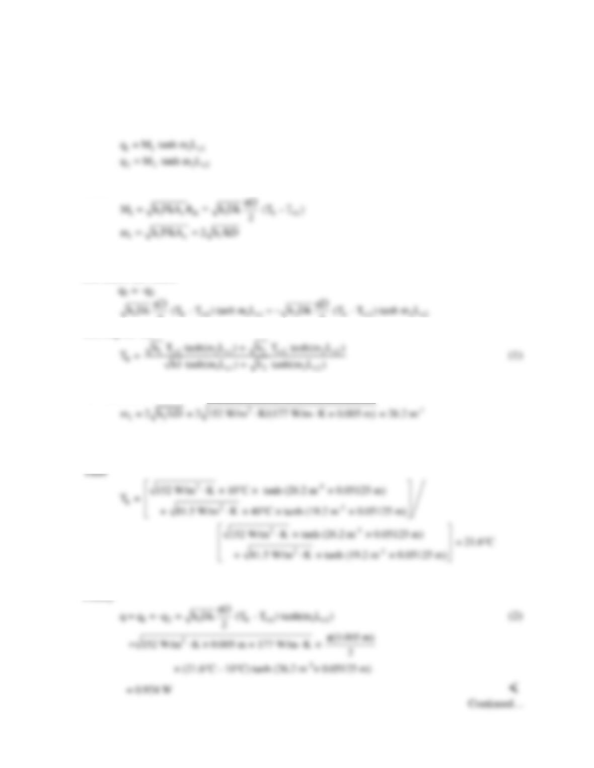
Next we analyze heat transfer along the rod as if it were two fins joined at their base – the location
where the fin passes through the wall. Thus, using the corrected fin length approach, Equation 3.94,
where
and Lci = Li + D/4. In this expression, L1 = d and L2 = L – d. Finally, since heat leaving one
rod enters the other,
22
Solving for Tb:
We calculate
and similarly, m2 = 19.2 m-1. Also, Lc1 = Lc2 = d + D/4 = 0.05 m + 0.005 m/4 = 0.05125 m.
Finally
PROBLEM 7.49 (Cont.)
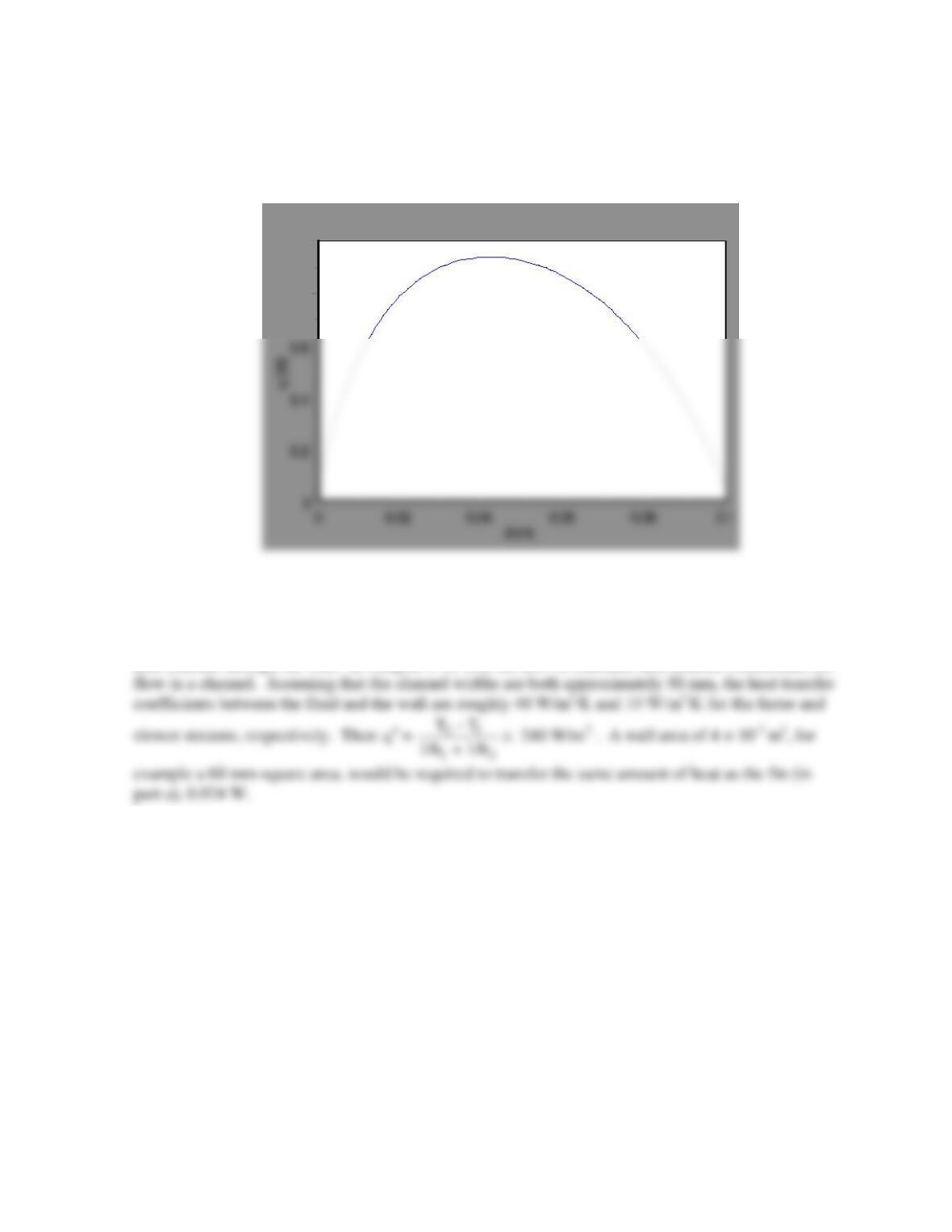
(b) With Lc1 = d + D/4 and Lc2 = L – d + D/4, we vary d in the range 0 ≤ d ≤ 0.1 m and solve
Equations (1) and (2). The results for q are plotted below.
1
0.8
We see that there is an optimal insertion distance, d
≅
40 mm. A longer fin length (≈ 60 mm) is
needed in fluid 2 to compensate for its smaller heat transfer coefficient.
COMMENTS: It is of interest to compare the heat transfer between the two fluids via the fin to the
heat transfer through the wall. In Chapter 8 we will see how to calculate heat transfer coefficients for
PROBLEM 7.50
KNOWN: Diameter and surface temperature of an uninsulated steam pipe. Velocity and temperature of
air in cross flow.
FIND: (a) Heat loss rate per unit length, (b) Effect of insulation thickness on heat loss rate.
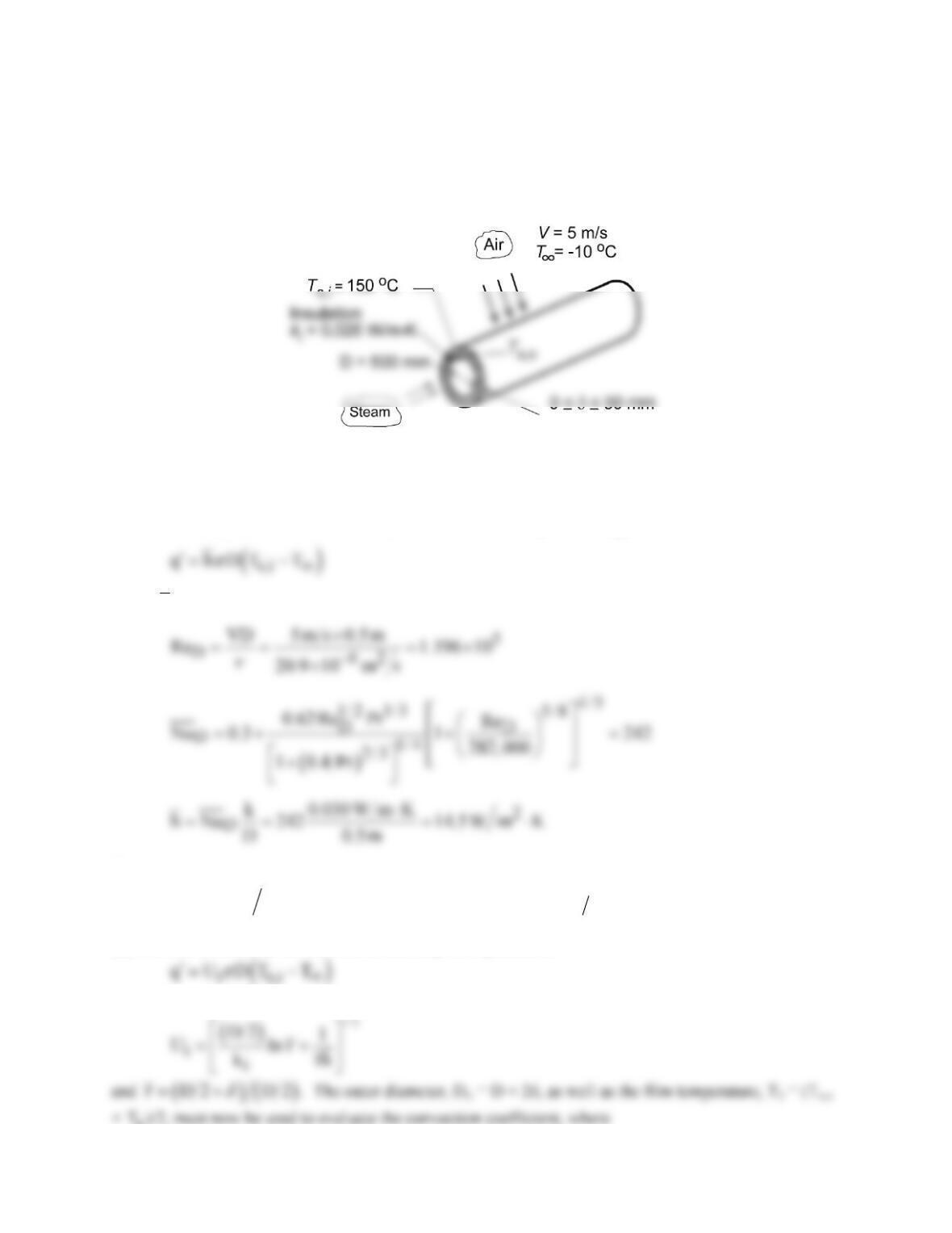
SCHEMATIC:
ASSUMPTIONS: (1) Steady-state conditions, (2) Uniform surface temperature, (3) Negligible
radiation.
PROPERTIES: Table A.4, Air (Tf ≈ 350 K, 1 atm): ν = 20.9 × 10⁻⁶ m2/s, k = 0.030 W/m⋅K, Pr = 0.70.
ANALYSIS: (a) Without the insulation, the rate of heat loss per unit length is
where
h
may be obtained from the Churchill-Bernstein relation. With
The heat rate is then
( ) ( )
( )
2
q 14.5 W m K 0.5m 150 10 C 3644 W m
π
′= ⋅ −− =
. <
(b) With the insulation, the rate of heat loss may be expressed as
where, from Eq. 3.36,
¥
Continued…
PROBLEM 7.50 (Cont.)
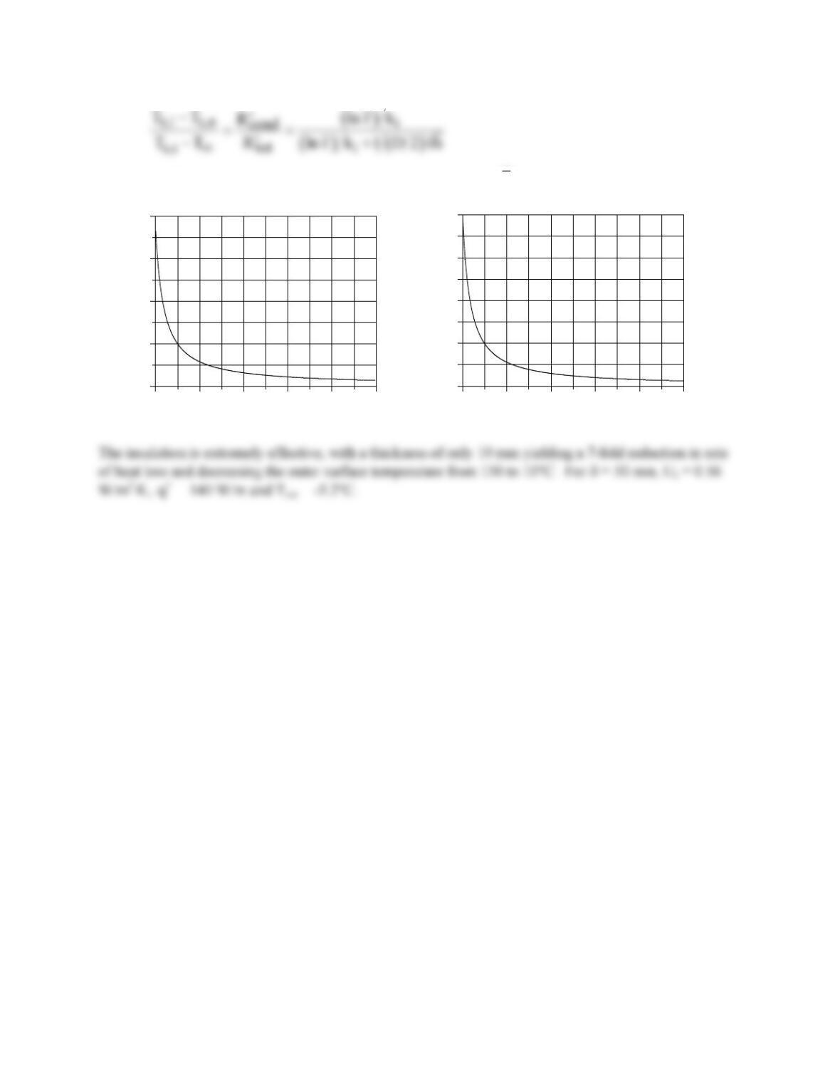
Using the IHT Correlations and Properties Tool Pads to evaluate
h
, the following results were obtained.
010 20 30 40 50
Insulation thickness, delta(mm)
0
1000
2000
3000
4000
Heat loss, q'(Ω/m)
010 20 30 40 50
Insulation thickness, delta(mm)
-10
10
30
50
70
90
110
130
150
Outer surface temperature, Tso(C)
COMMENTS: The dominant contribution to the total thermal resistance is made by the insulation.
PROBLEM 7.51
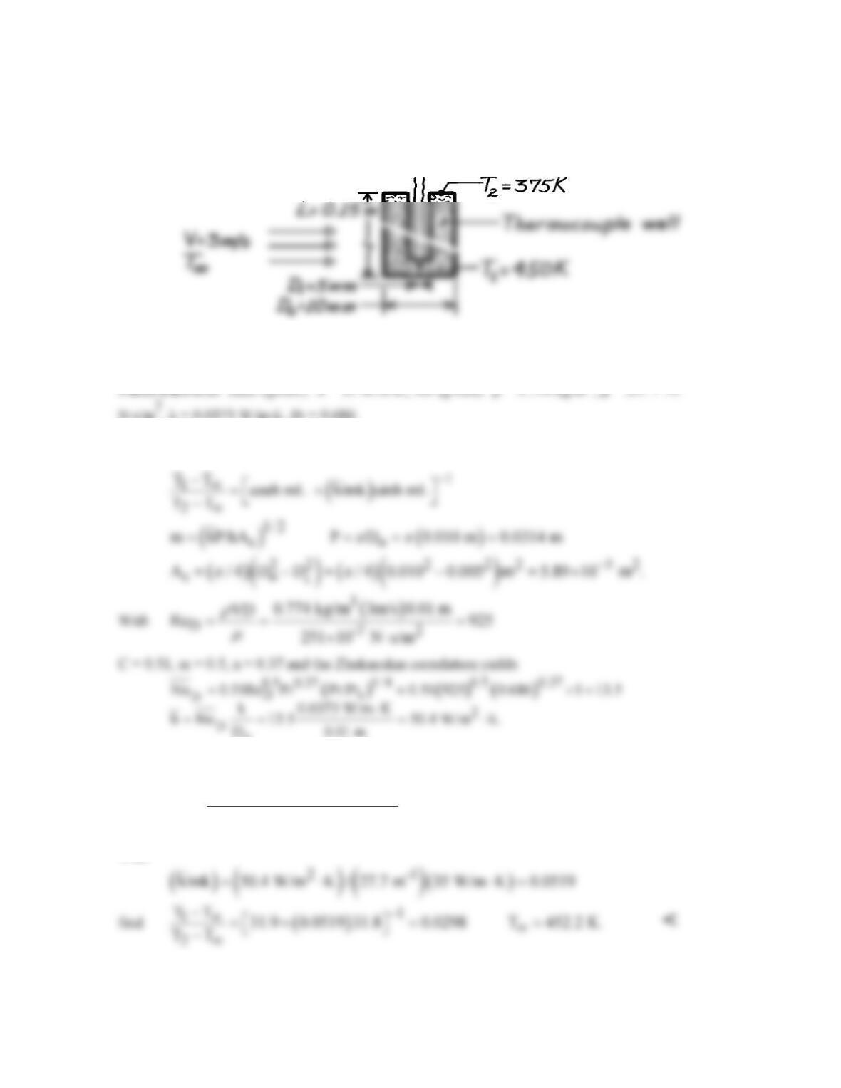
KNOWN: Dimensions and thermal conductivity of a thermocouple well. Temperatures at well tip
and base. Air velocity.
FIND: Air temperature.
SCHEMATIC:
ASSUMPTIONS: (1) Steady-state conditions, (2) Constant properties, (3) One-dimensional
conduction along well, (4) Uniform convection coefficient, (5) Negligible radiation.
N⋅s/m2, k = 0.0373 W/m⋅K, Pr = 0.686.
ANALYSIS: Applying Equation 3.75 at the well tip (x = L), where T = T1,
o
Hence
()
( )
()
1/ 2
2
-1 -1
52
50.4 W/m K 0.0314 m
m 27.7 m mL 27.7 m 0.15 m 4.15.
35 W/m K 5.89 10 m
−
⋅
= = = =
⋅×
With
COMMENTS: Heat conduction along the wall to the base at 375 K is balanced by convection from
the air.
PROBLEM 7.52
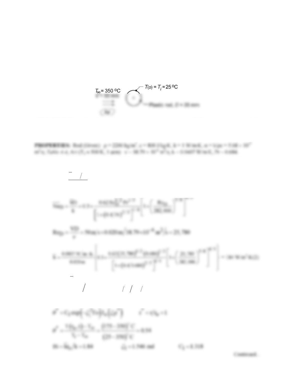
KNOWN: Long coated plastic, 20-mm diameter rod, initially at a uniform temperature of Ti = 25°C, is
suddenly exposed to the cross–flow of air at
T∞
= 350°C and V = 50 m/s.
FIND: (a) Time for the surface of the rod to reach 175°C, the temperature above which the special
coating cures, and (b) Compute and plot the time-to–reach 175°C as a function of air velocity for 5 ≤ V ≤
50 m/s.
SCHEMATIC:
ASSUMPTIONS: (a) One-dimensional, transient conduction in the rod, (2) Constant properties, and (3)
Evaluate thermophysical properties at Tf = [(Ts + Ti)/2 +
T
∞
]/2 = [(175 + 25)/2 + 350]°C/2 = 225°C =
500 K.
ANALYSIS: (a) To determine whether the lumped capacitance method is valid, determine the Biot
number
( )
o
lc
hr 2
Bi k
=
(1)
The convection coefficient can be estimated using the Churchill-Bernstein correlation, Eq. 7.54,
Substituting for
h
from Eq. (2) into Eq. (1), find
( )
2
lc
Bi 184 W m K 0.010 m 2 1W m K 0.92 0.1= ⋅ ⋅ = >>
Hence, the lumped capacitance method is inappropriate. Using the one-term series approximation, Eqs.
5.52 with Table 5.1,
PROBLEM 7.52 (Cont.)
0.54 = 1.318exp[-(1.546rad)2Fo]Jo(1.546 × 1)
Using Table B.4 to evaluate Jo(1.546) = 0.4859, find Fo = 0.0725 where
o
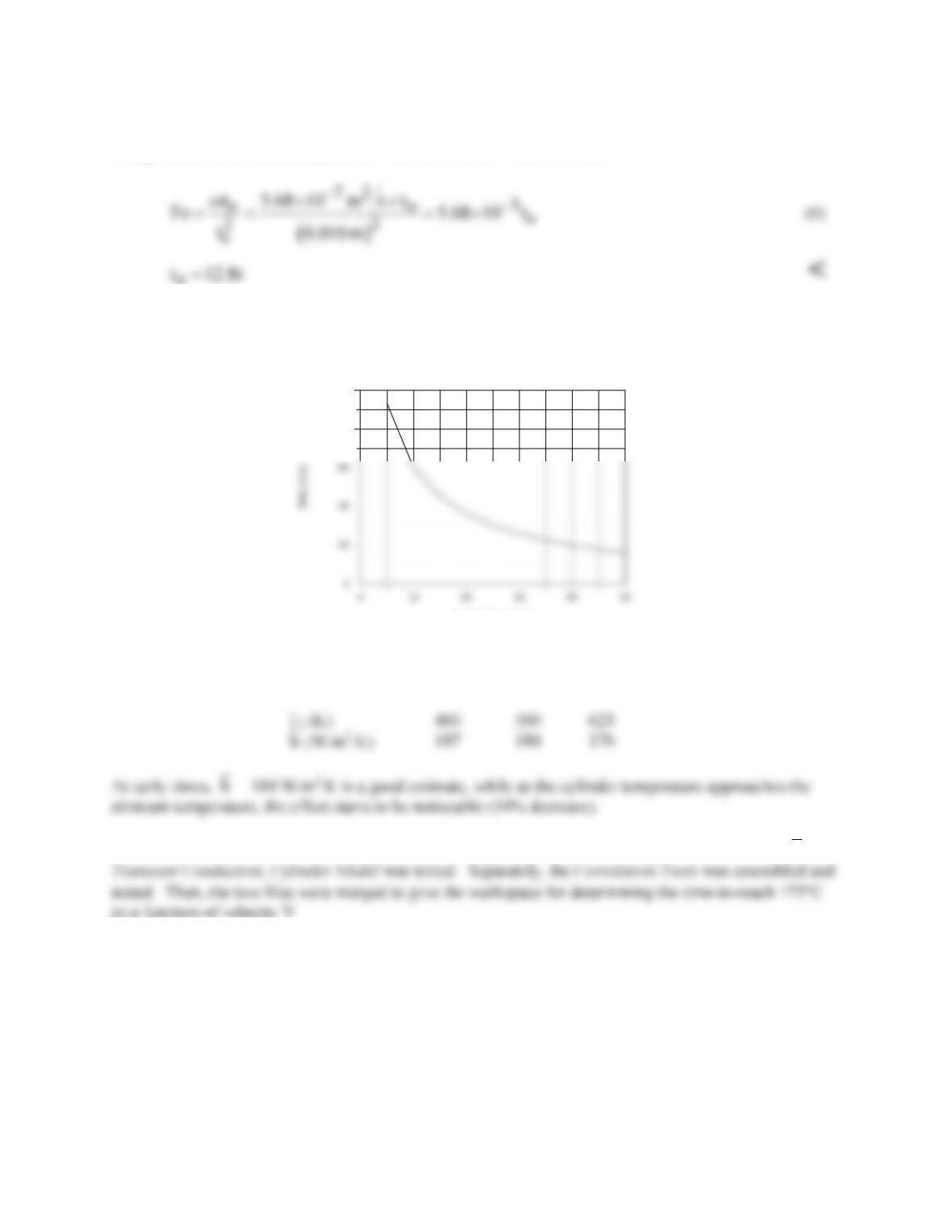
(b) Using the IHT Model, Transient Conduction, Cylinder, and the Tool, Correlations, External Flow,
Cylinder, results for the time–to–reach a surface temperature of 175°C as a function of air velocity V are
plotted below.
Air velocity, V (m/s)
80
100
COMMENTS: (1) Using the IHT Tool, Correlations, External Flow, Cylinder, the effect of the film
temperature Tf on the estimated convection coefficient with V = 50 m/s can be readily evaluated.
(2) The IHT analysis performed for part (b) was developed in two parts. Using a known value for
h
, the
PROBLEM 7.53
KNOWN: Velocity, diameter, initial temperature and properties of extruded wire. Temperature and
velocity of air. Temperature of surroundings.
FIND: (a) Differential equation for temperature distribution T(x), (b) Exact solution for negligible
radiation and corresponding value of temperature at prescribed length of wire, (c) Effect of radiation
on temperature of wire at prescribed length. Effect of wire velocity and emissivity on temperature
distribution.
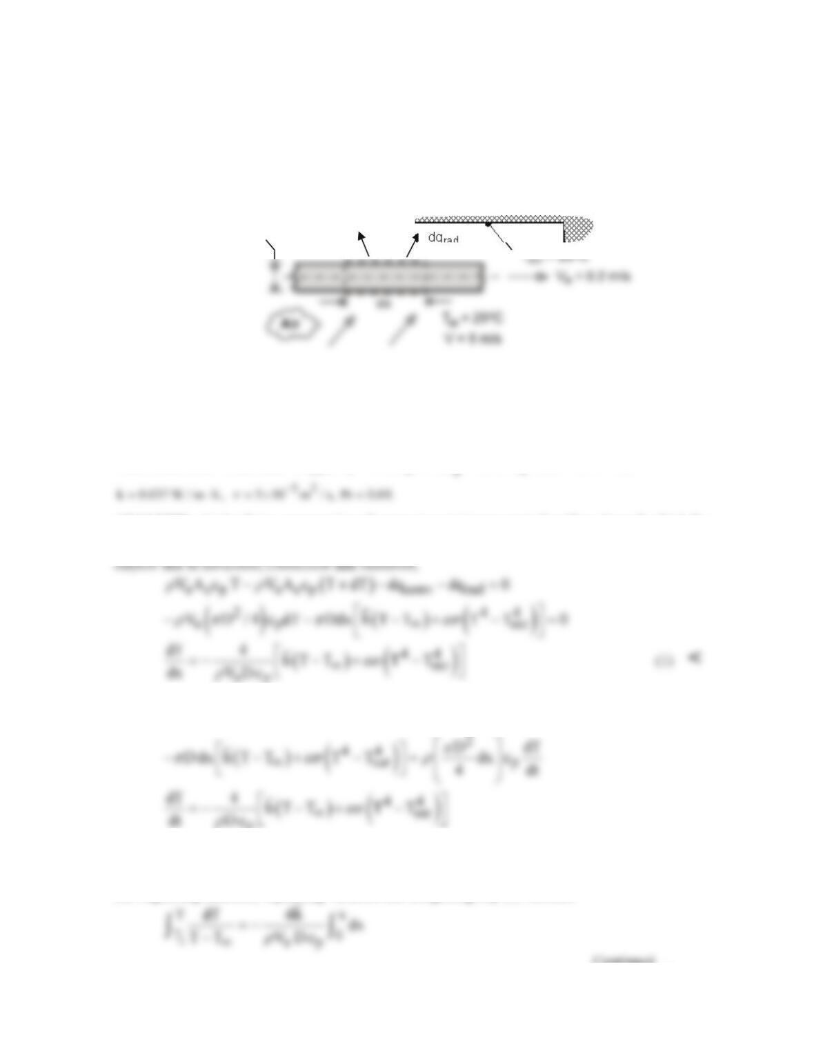
SCHEMATIC:
dq
rad
dq
conv
D = 5 mm
ASSUMPTIONS: (1) Negligible variation of wire temperature in radial direction, (2) Negligible
effect of axial conduction along the wire, (3) Constant properties, (4) Radiation exchange between
small surface and large enclosure, (5) Motion of wire has a negligible effect on the convection
coefficient (Ve << V).
PROPERTIES: Prescribed. Copper:
3
p
8900 kg / m , c 400 J / kg K, 0.55.
ρε
= = ⋅=
Air:
ANALYSIS: (a) Applying conservation of energy to a stationary control surface, through which the
wire moves, steady–state conditions exist and
in out
E E 0.−=
Hence, with inflow due to advection and
Alternatively, if the control surface is fixed to the wire, conditions are transient and the energy
balance is of the form,
out st
E E,−=
or
p
Dividing the left– and right-hand sides of the equation by dx/dt and
e
V dx / dt,=
respectively, Eq. (1)
is obtained.
(b) Neglecting radiation, separating variables and integrating, Eq. (1) becomes
Continued …
PROBLEM 7.53 (Cont.)
With
52
D
Re VD / 5 m / s 0.005 m / 3 10 m / s 833,
ν
−
==×× =
the Churchill-Bernstein correlation yields
Hence, applying Eq. (2) at x = L,
o
o
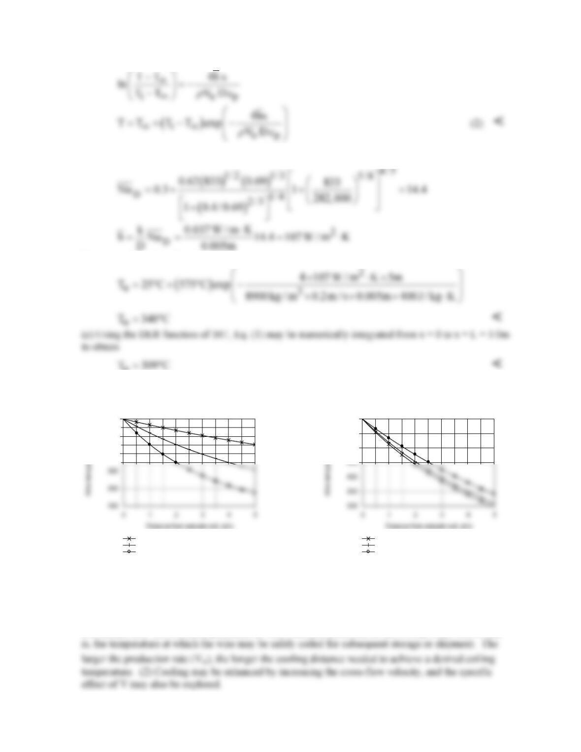
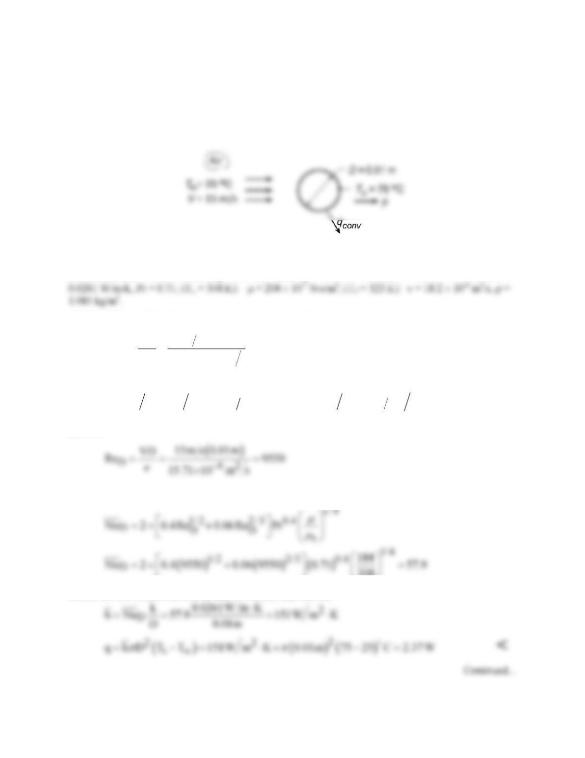
Hence, radiation makes a discernable contribution to cooling of the wire. IHT was also used to obtain
the following distributions.
The speed with which the wire is drawn from the extruder has a significant influence on the
temperature distribution. The temperature decay decreases with increasing Ve due to the increasing
effect of advection on energy transfer in the x direction. The effect of the surface emissivity is less
pronounced, although, as expected, the temperature decay becomes more pronounced with increasing
ε.
COMMENTS: (1) A critical parameter in wire extrusion processes is the coiling temperature, that
400
500
600
Ve=0.5 m/s
Ve=0.2 m/s
Ve=0.1 m/s
500
550
600
eps=0.8
eps=0.55
eps=0
PROBLEM 7.54
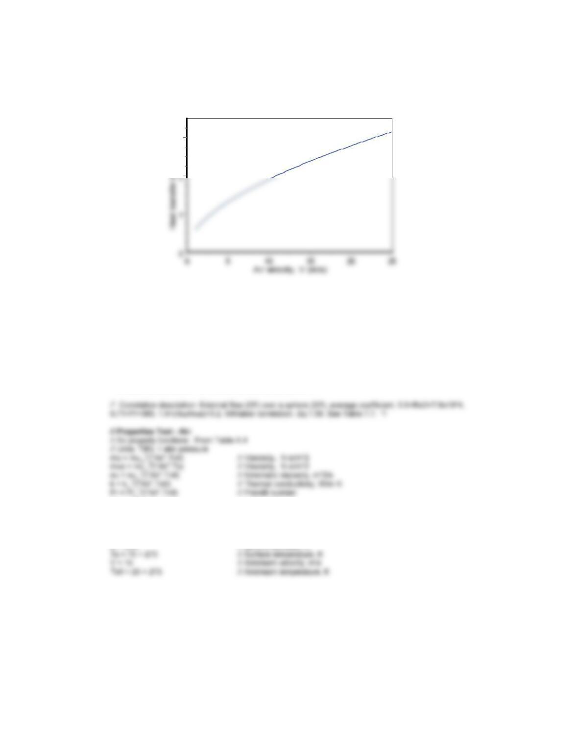
KNOWN: Temperature and velocity of air flow over a sphere of prescribed surface temperature and
diameter.
FIND: (a) Drag force, (b) Heat transfer rate with air velocity of 15 m/s; and (c) Compute and plot the
heat rate as a function of air velocity for the range 1 ≤ V ≤ 25 m/s.
SCHEMATIC:
ASSUMPTIONS: (1) Steady-state conditions, (2) Uniform surface temperature, (3) Negligible radiation
exchange with surroundings.
PROPERTIES: Table A.4, Air (
T¥
= 298 K, 1 atm): µ = 184 × 10-7 N⋅s/m2; ν = 15.71 × 10⁻⁶ m2/s, k =
ANALYSIS: (a) Working with properties evaluated at Tf
( )
D62
15m s 0.01m
VD
Re 8240
18.2 10 m s
ν
−
= = =
×
and from Fig. 7.9, find CD ≈ 0.4. Hence
()()
( )( ) ( )
22
22 3
DD
F C D 4 V 2 0.4 4 0.01m 1.085kg m 15m s 2 0.0038 N
πρ π
= = =
<
(b) With
it follows from the Whitaker relation that
208
Hence, the convection coefficient and convection heat rate are
PROBLEM 7.54 (Cont.)
(c) Using the IHT Correlation Tool, External Flow, Sphere, the heat rate was calculated and is plotted
below.
3
COMMENTS: (1) The Whitaker correlation is valid for
s
/
µµ
> 1, whereas the value here is 0.89,
slightly outside of the allowable range. (2) A copy of the IHT Workspace used to generate the above plot
is shown below.
// Correlation Tool – External Flow, Sphere:
NuDbar = NuL_bar_EF_SP(ReD,Pr,mu,mus) // Eq 7.56
NuDbar = hbar * D / k
ReD = V * D / nu
/* Evaluate properties at Tinf and the surface temperature, Ts. */
// Heat Rate Equation:
q = hbar * pi * D^2 * (Ts – Tinf)
// Assigned Variables:
PROBLEM 7.55
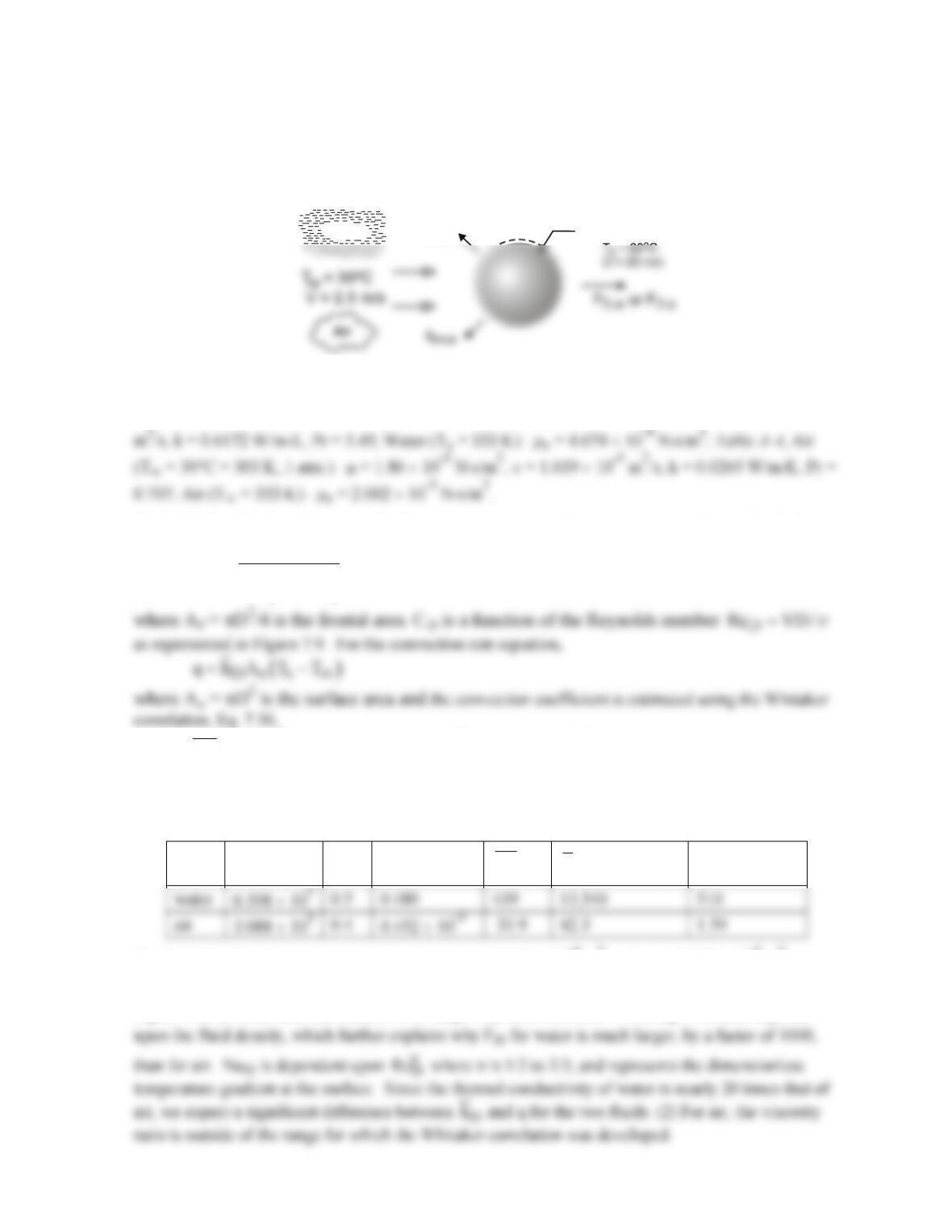
KNOWN: Sphere with a diameter of 20 mm and a surface temperature of 60°C that is immersed in a
fluid at a temperature of 30°C with a velocity of 2.5 m/s.
FIND: The drag force and the heat rate when the fluid is (a) water and (b) air at atmospheric pressure.
Explain why the results for the two fluids are so different.
SCHEMATIC:
Water
q
cv,w
Sphere
ASSUMPTIONS: (1) Flow over a smooth sphere, (2) Constant properties.
PROPERTIES: Table A-6, Water (T∞ = 30°C = 303 K): µ = 8.034 × 10⁻⁴ N⋅s/m2, ν = 8.068 × 10⁻⁷
ANALYSIS: The drag force, Fo, for the sphere is determined from the drag coefficient, Eq. 7.50,
()
D
D2
f
F
C
A V /2
ρ
=
( )
D
1/4
1/ 2 2 / 3 0.4 s
DD
Nu 2 0.4 Re 0.06 Re Pr /
µµ
=++
where all properties except µs are evaluated at T∞. For convenience we will evaluate properties
required for the drag force at T∞. The results of the analyses for the two fluids are tabulated below. <
Fluid ReD CD FD (N)
D
Nu
()
2
D
h W/m K⋅
q(W)
The frontal and surface areas, respectively, are Af = 3.142 × 10⁻⁴ m2 and As = 1.257 × 10⁻³ m2.
COMMENTS: (1) The Reynolds number is the ratio of inertia to viscous forces. We associate
higher viscous shear and heat transfer with larger Reynolds numbers. The drag force also depends
PROBLEM 7.56
KNOWN: An underwater instrument pod having a spherical shape with a diameter of 100 mm
dissipating 400 W.
FIND: Estimate the surface temperature of the pod for these conditions: (a) when submersed in a bay
where the water temperature is 15°C and the current is 1 m/s, and (b) after being hauled out of the
water without deactivating the power and suspended in the ambient where the air temperature is 15°C
and the wind speed is 3 m/s.
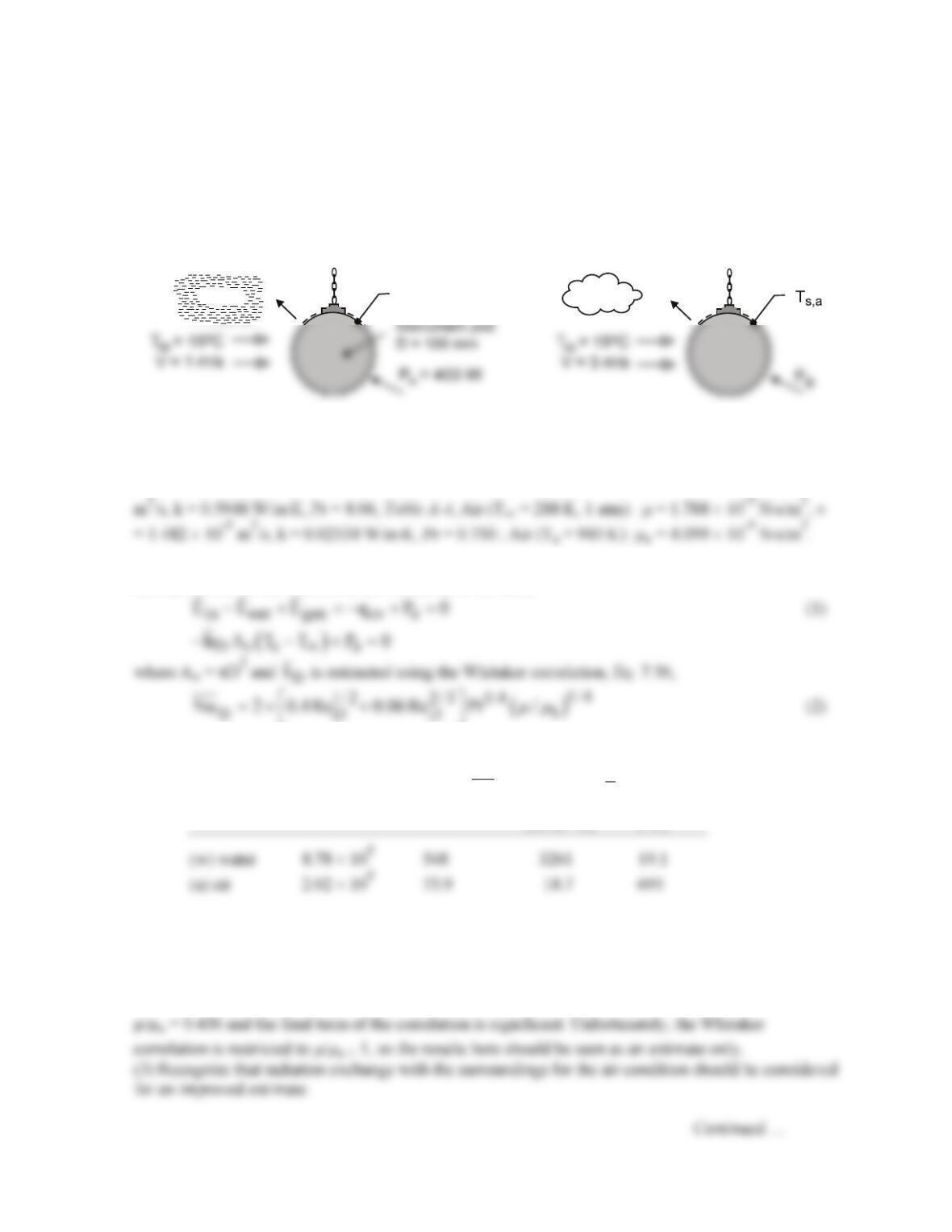
SCHEMATIC:
Water
Ambient
air
T
s,w
q
cv
q
cv
ASSUMPTIONS: (1) Steady–state conditions, (2) Flow over a smooth sphere, (3) Uniform surface
temperatures, (4) Negligible radiation heat transfer, and (5) Constant properties (µ = µs) for water.
PROPERTIES: Table A-6, Water (T∞ = 15°C = 288 K): µ = 0.001053 N⋅s/m2, ν = 1.139 × 10⁻⁶
ANALYSIS: The energy balance for the submersed–in–water (w) and suspended-in–air (a) conditions
are represented in the schematics above and have the form
D
where all properties except µs are evaluated at T∞. The results are tabulated below.
Condition ReD
D
Nu
D
h
Ts
(W/m2⋅K) (°C)
COMMENTS: (1) While submerged and dissipating 400 W, the pod is safely operating at a
temperature slightly above that of the water. When hauled from the water and suspended in air, the
pod temperature increases to a destruction temperature (695°C).
(2) The assumption that µ/µs ≈ 1 is appropriate for the water (w) condition. For the air (a) condition,

PROBLEM 7.56 (Cont.)
(4) Why is there such a difference in Ts for the water (w) and air (a) conditions? From the results
table note that the ReD, NuD, and
D
h
are, respectively, 4x, 7x and 170x times larger for water
compared to air. Water, because of its thermophysical properties which drive the magnitude of
D
h,
is
a much better coolant than air for similar flow conditions.
// Correlation, sphere
NuDbar = NuL_bar_EF_SP(ReD,Pr,mu,mus) // Eq 7.56
NuDbar = hbar * D / k
// Input variables
D = 0.1
//V = 1.0 // Ωater current
V = 3 // Ωind speed
Tinf_C = 15
Pelec = 400
// Conversions
Tinf = Tinf_C + 273
Ts = Ts_C + 273