Problem 6.16
The stream function for an incompressible, two-dimensional flow field is
3
ay by
ψ
=−
where
a
and
b
are constants. Is this an irrotational flow? Explain.
Solution 6.16
For the flow to be irrotational,
10
2
z
vu
xy
ω
∂∂
=−=
∂∂
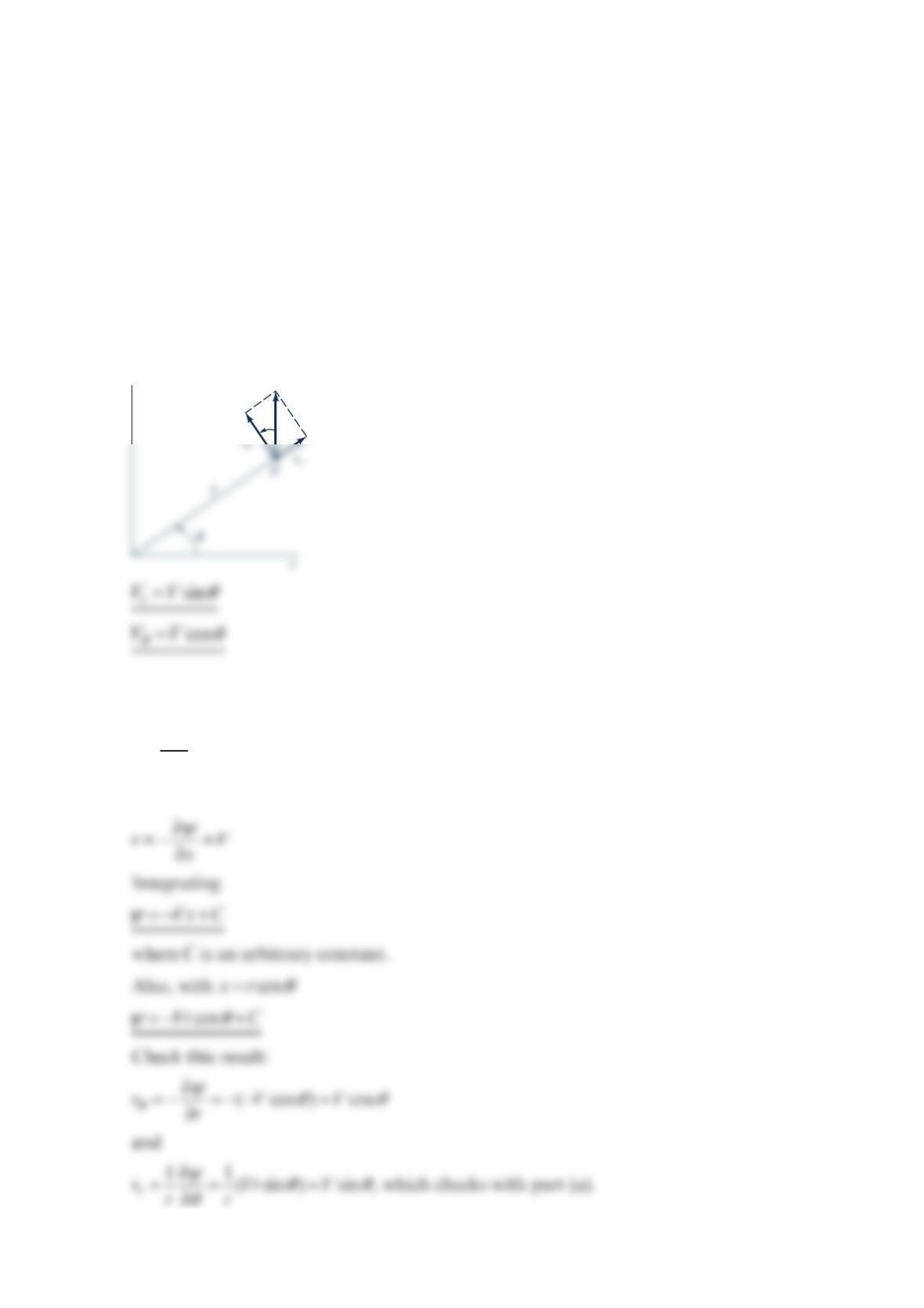
Problem 6.17
For a certain two-dimensional flow field
0u=
uV=
(a) What are the corresponding radial and tangential velocity components? (b) Determine
the corresponding stream function expressed in Cartesian coordinates and in cylindrical po-
lar coordinates.
Solution 6.17
(a) At an arbitrary point P (see figure)
(b) Since
0u
y
ψ
∂
==
∂
It follows that
ψ
is not a function of
y
and
y
θ
V
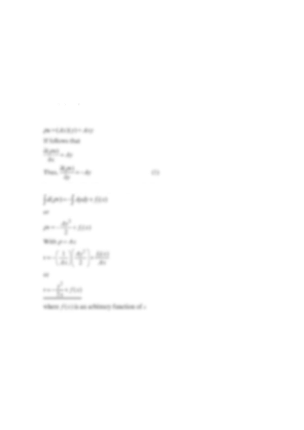
Problem 6.18
In a certain steady, two-dimensional flow field, the fluid density varies linearly with respect
to the coordinate x: that is, A
x
ρ
= where
A
is a constant. If the x component of velocity
u
is
given by the equation u
y
=, determine an expression for
v
.
Solution 6.18
For a variable density flow,
() ()
0
uv
xy
ρρ
∂∂
+=
∂∂
With
Integrate Eq. (1) with respect to
y
to obtain
ρ
x
ρ
ρ
y
ρ
Problem 6.19
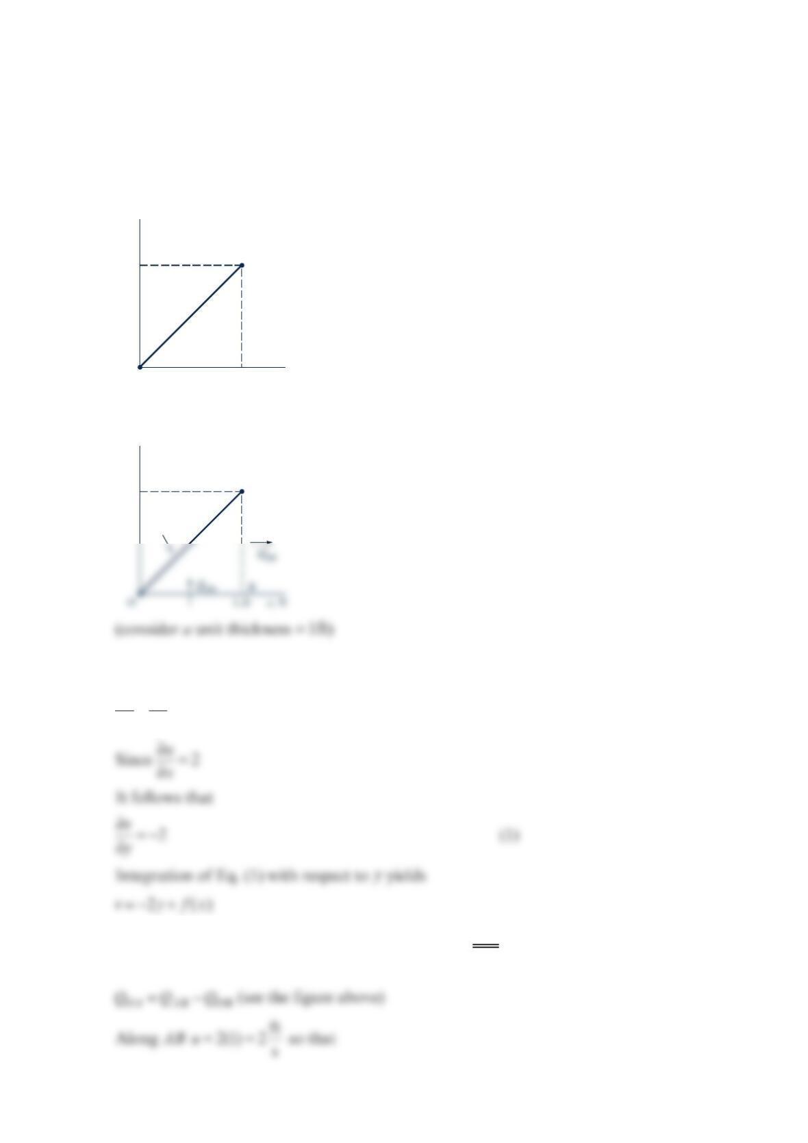
In a two-dimensional, incompressible flow field, the x component of velocity is given by the
equation 2u
x
=. (a) Determine the corresponding equation for the y component of velocity
if 0v= along the x axis. (b) For this flow field, what is the magnitude of the average velocity
of the fluid crossing the surface O
A
of the figure below? Assume that the velocities are in
feet per second when x and
y
are in feet.
Solution 6.19
(a) To satisfy the continuity equation
0
uv
xy
∂∂
+=
∂∂
y
If 0v= along -axi
s
x
(
0)
y
= then ( ) 0
f
x= so that 2vy=−
(b) To satisfy conservation of mass
A
O
y
, ft
x, ft1.0
1.0
A
Q
OA
y
, ft
1.0
3
ft ft
2(1ft)(1ft)2
ss
AB AB
QuA
== =
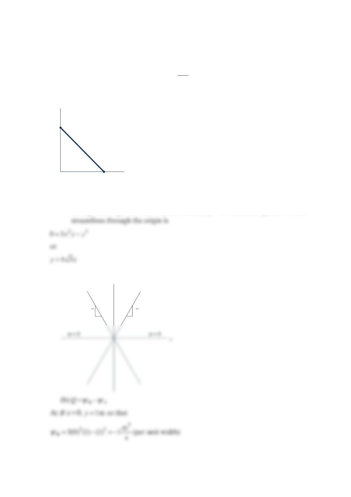
Problem 6.20
The stream function for an incompressible flow field is given by the equation
23
3xy y
ψ
=−
where the stream function has the units of
2
m
s with x and y in meters. (a) Sketch the
streamline(s) passing through the origin. (b) Determine the rate of flow across the straight
path AB shown in the figure below.
Solution 6.20
(a) Lines of constant
ψ
are streamlines. For 23
3xy y
ψ
=−
, the streamline passing
through the origin ( 0x=, 0
y
=) has the value 0
ψ
=. Thus, the equation for the
A sketch of these streamlines is shown in the figure below.
y
y
, m
x
, m1.0
1.0
B
A
0
11
y
= 0
√3
√3
ψ
= 0
ψ
y
At A 1
m
x= , 0
y
= so that
23
3(1) (0) (0) 0
A
ψ
=−=
Thus,
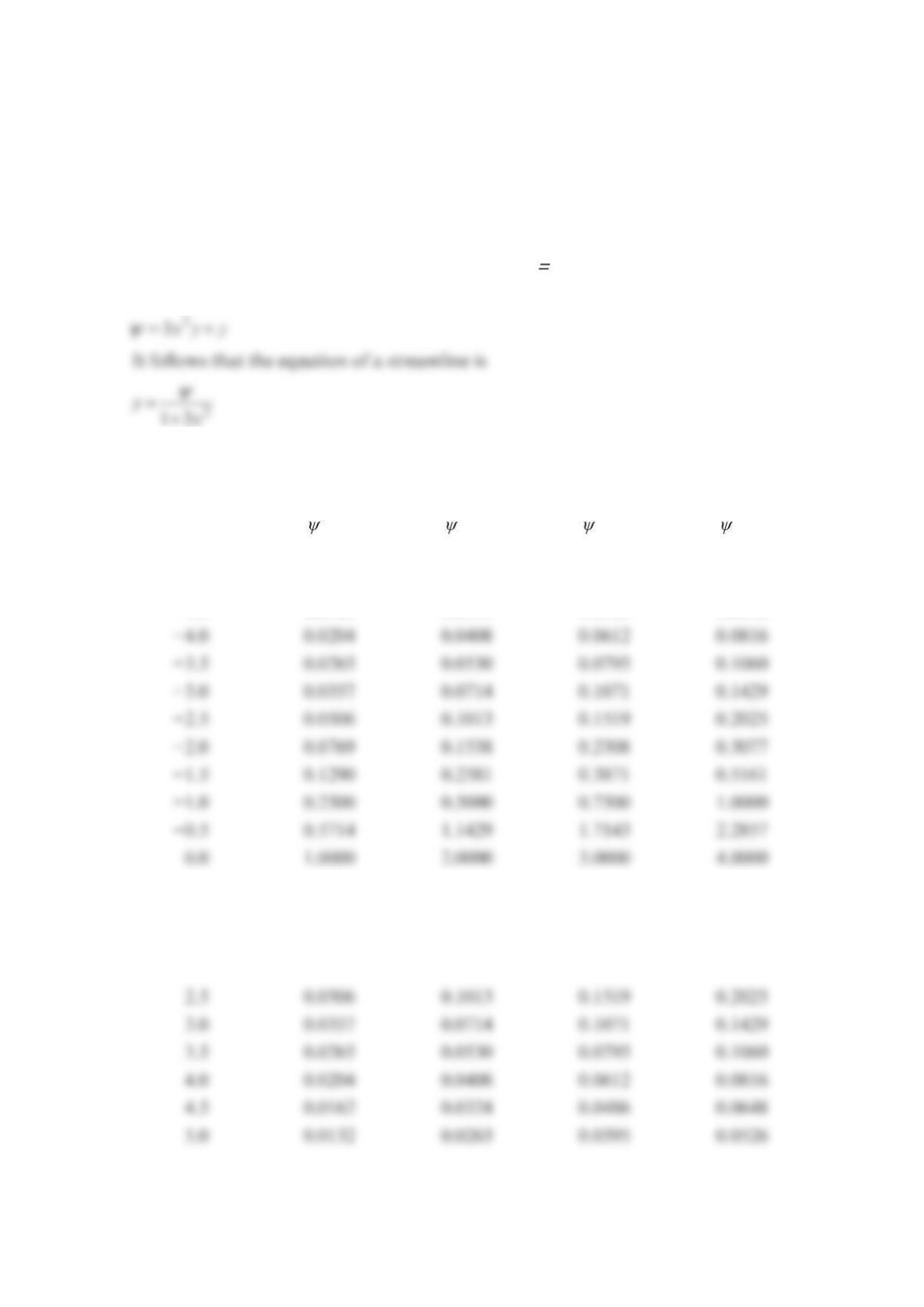
Problem 6.21
The stream function for an incompressible, two-dimensional flow field is
2
3xy y
ψ
=+
For this flow field, plot several streamlines.
Solution 6.21
The equation for a streamline is found by setting constant
ψ
in the equation for the
stream function. Thus, for the given stream function.
where various constant values can be assigned to
ψ
to obtain a family of streamlines. Tabu-
lated results for 1,2,3, 4,
ψ
= and a plot showing the streamlines are given below.
= 1 = 2 = 3 = 4
x y y y y
−5.0 0.0132 0.0263 0.0395 0.0526
−4.5 0.0162 0.0324 0.0486 0.0648
0.5 0.5714 1.1429 1.7143 2.2857
1.0 0.2500 0.5000 0.7500 1.0000
1.5 0.1290 0.2581 0.3871 0.5161
2.0 0.0769 0.1538 0.2308 0.3077
ψ
3.00
3.50
4.00
4.50
= 3
ψ
= 4
ψ
= 3
ψ
= 4
ψ
Problem 6.22
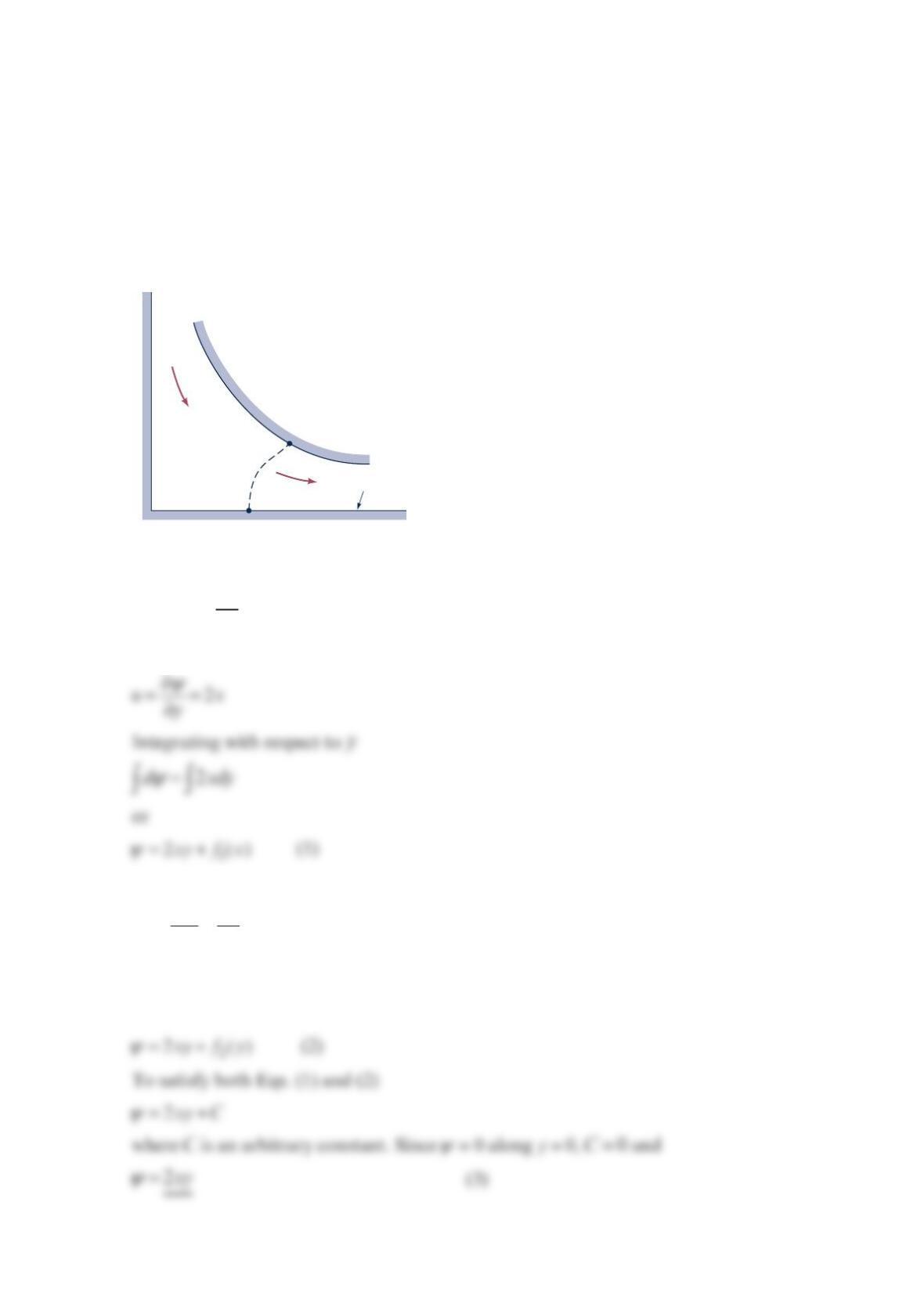
Consider the incompressible, two-dimensional flow of a nonviscous fluid between the
boundaries shown in the figure below. The velocity potential for this flow field is
22
xy
φ
=−
(a) Determine the corresponding stream function. (b) What is the relationship between the
discharge,
q
(per unit width normal to plane of paper) passing between the walls and the
coordinates i
x
, i
y
of any point on the curved wall? Neglect body forces.
Solution 6.22
(a) 2ux
x
φ
∂
==
∂
In terms of the stream function,
Similarly,
2vy
xy
ψφ
∂∂
=− = =−
∂∂
So that 2dyd
x
ψ
=
or
y
x
A
B
q
q
ψ
= 0
(
xi
,
yi
)
ψ
ψ
(b) The discharge,
q
, passing through any surface connecting the two walls, such as
AB
(see figure), is
Problem 6.23
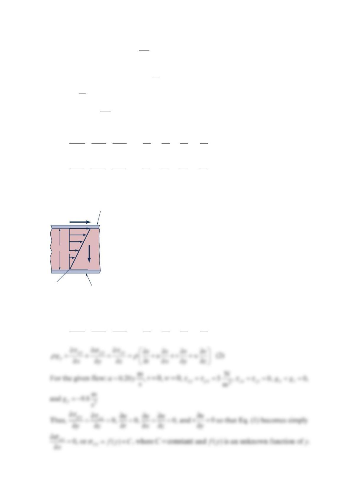
A fluid with a density of 3
kg
2
000 m
flows steadily between two flat plates as shown in the fig-
ure below. The bottom plate is fixed and the top one moves at a constant speed in the x di-
rection. The velocity is m
ˆ
0.20 s
y= Vi
where y is in meters. The acceleration of gravity is
2
m
ˆ
9.8 s
=− gj
. The only nonzero shear stresses, yx xy
τ
τ
=, are constant throughout the flow
with a value of 2
N
5
m
. The normal stress at the origin
(
0)xy== is 100 kPa
xx
σ
=− . Use the
x and
y
components of the equations of motion
yx
xx zx
x
uuu u
guvw
xyz txyz
τ
στ
ρρ
∂
∂∂
∂∂∂ ∂
+++= +++
∂∂∂ ∂∂∂∂
xy yy zy
y
vvv v
guvw
xyz txyz
τστ
ρρ
∂∂ ∂
∂∂∂ ∂
++ += +++
∂∂∂ ∂∂∂∂
to determine the normal stress throughout the fluid. Assume that xx yy
σ
σ
=.
Solution 6.23
yx
xx zx
x
uuu u
guvw
xyz txyz
τ
στ
ρρ
∂
∂∂
∂∂∂ ∂
+++= +++
∂∂∂ ∂∂∂∂
(1)
U
Moving
plate
Fixed
plate
b
z
x
yg
τ
Similarly, since yy xx
σ
σ
=, Eq. (1) becomes:
but
xx
f
y
y
σ
∂∂
=
∂∂
so that
f
Problem 6.24
In Section 6.3, we derived the differential equation(s) of linear momentum by considering
the motion of a fluid element. Derive the linear momentum equation(s) by considering a
small control volume, like we did for the continuity equation in Section 6.2.
Solution 6.24
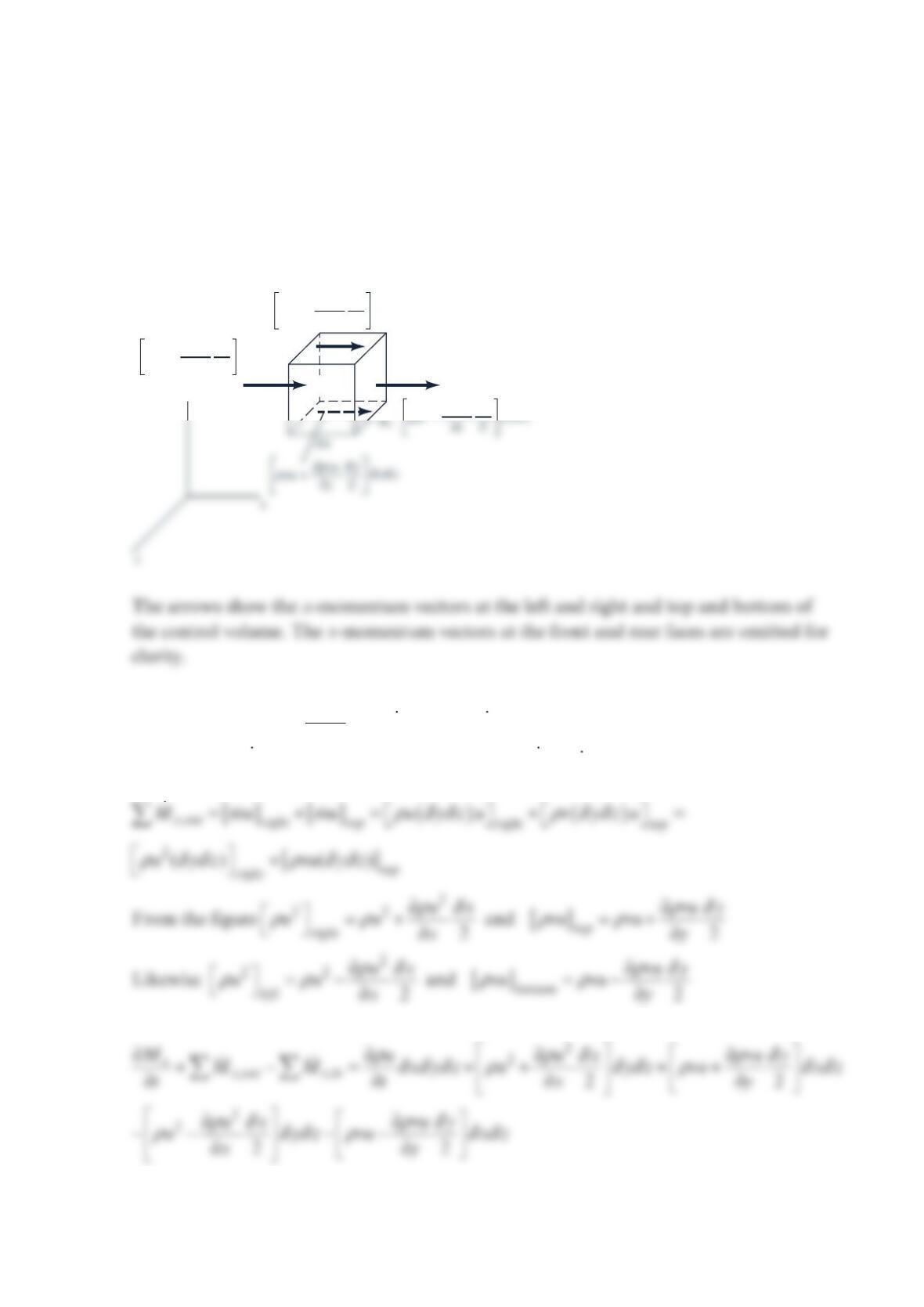
Consider the differential control volume shown below (adapted from Fig. 6.5)
For a control volume ,,
xxout xin x
MMMF
t
∂+−=
∂
where x
M
is the x-momentum;
x
M
mu= and x
M
is the flowrate of x-momentum; x
M
mu=. For the infinitesimal control
volume, ()
x
M
xyzu
ρ
δδδ
= and
Then
2
– 2
u
2
ρ∂
u
2
ρ∂
x
δ
vu
+ 2
ρ
vu
ρ∂
v
∂
xz
δδ
y
δ
u
2
–
2
ρ
u
2
ρ
x
∂
yz
δδ
y
y
δ
x
δ
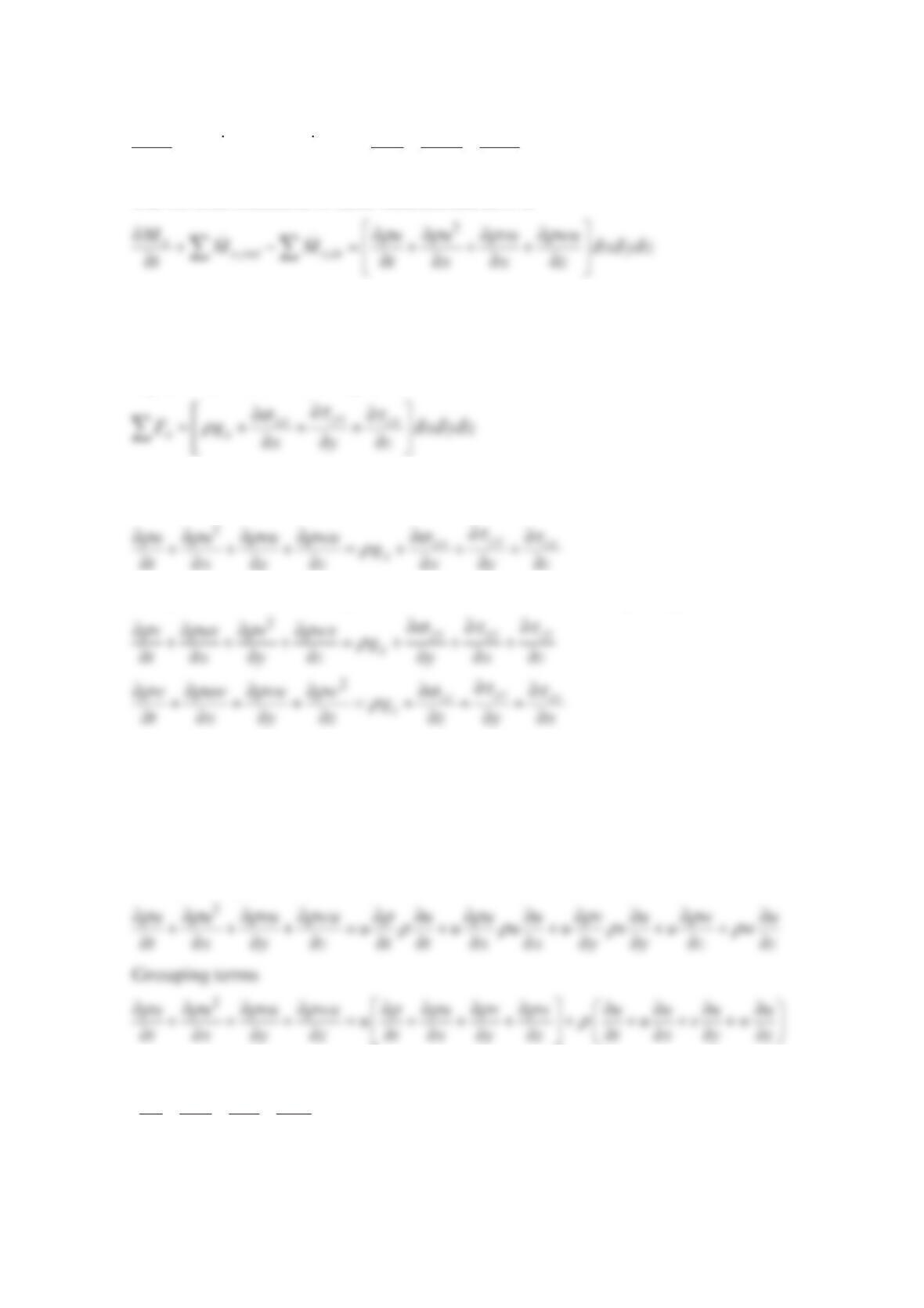
Cancelling and collecting terms
2
,,
xx out x in
Muu vu
MM xyz
ttxx
ρρ ρ
δδδ
∂∂∂ ∂
+−=++
∂∂∂∂
The obvious extension to three-dimensional flow is
The sum of the forces acting on the cube of fluid inside the control volume is identical to
the sum of forces when the cube is considered to be an individual particle and is given by
Eq. (6.50a) and shown in Fig. 6.11
Assembling the momentum equation and dividing by xyz
δ
δδ
gives the x-momentum equa-
tion for three-dimensional flow.
The y– and z-momentum equations are derived in the same way. They are
These equations are not identical to Eqs. (6.50). The momentum equations here are said to
be in conservative form. This form is most suitable for Computational Fluid Dynamics
(CFD). See Appendix A.
To illustrate the equivalence of the conservative form with Eqs. (6.50), consider the x–
momentum equation. The difference is on the left (acceleration) side only. Using the Prod-
uct Rule for Differentiation:
According to the continuity equation [Eq. (6.27)]
0
uvw
tx y z
ρρ ρ ρ
∂∂ ∂ ∂
+++ =
∂∂ ∂ ∂
yx
xx zx
x
uuu u
uvw g
txyz x y z
τ
στ
ρρ
∂
∂∂
∂∂∂ ∂
+++ =+ + +
∂∂∂ ∂ ∂ ∂ ∂
which are equivalent to Eqs. (6.50). Options for the stress terms on the right side are the
same as those discussed in Chapter 6 for laminar flow and Appendix A for turbulent flow.
Problem 6.25
By considering the rotational equilibrium of a fluid mass element, show that .
xy yx
τ
τ
=
Solution 6.25
The sketch shows the stresses in the x
y
− plane acting on a fluid particle.
Apply Newton’s second law in rotational form
zz
z
MI
ω
=
where z
M
is the moment about the z axis (perpendicular to the paper, passing through the
center of the element), z
I
the moment of inertia, and z
ω
τ
xy
τ
yy
σ
yx
τ
Problem 6.26
The stream function for a given two-dimensional flow field is
23
55xy y
ψ
=−
Determine the corresponding velocity potential.
Solution 6.26
22
55uxy
y
x
ψφ
∂∂
===−
∂∂ (1)
Similarly,
Problem 6.27
A certain flow field is described by the stream function
sinABr
ψ
θ
θ
=+
where A and B are positive constants. Determine the corresponding velocity potential and
locate any stagnation points in this flow field.
Solution 6.27
1cos
r
A
vB
rrr
ψφ
θ
θ
∂∂
===+
∂∂ (1)
Integrate with respect to r to obtain
Similarly,
θ
where C is an arbitrary constant.
Stagnation points occur where 0
r
v= and 0
v
θ
=.
From Eq. (3), 0
v
θ
= at
0
θ
= and
θπ
=. From Eq. (1), with
0
θ
=
r
A
vB
r
=+
θπ
Problem 6.28
Integrate Bernoulli’s equation for compressible flow,
2
constant
2
dp V gz
ρ
++=
,
for an ideal gas undergoing an isothermal (constant temperature) process along a stream-
line.
Solution 6.28
The equation along a streamline is
2
2
dp V gz C
ρ
++=