Chapter 6 This is consistent with the fact that the surface

PROBLEM 6.1

KNOWN: Temperature distribution at x2 in laminar thermal boundary layer.

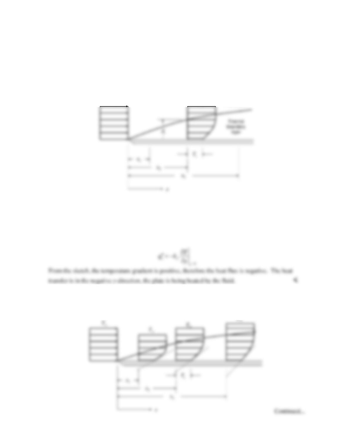
FIND: (a) Whether plate is being heated or cooled, (b) Temperature distributions at two other x

locations. Locations of largest and smallest heat fluxes, (c) Temperature distribution at x2 for lower

and higher free stream velocities. Which velocity condition causes the largest heat flux.

SCHEMATIC:

T

∞

T

∞

Free stream

ASSUMPTIONS: (1) Steady-state conditions, (2) Laminar, incompressible flow.

ANALYSIS: (a) Since the sketch indicates that the free stream temperature is greater than the

surface temperature, the plate is being heated by the fluid. This is consistent with the fact that the

surface heat flux in the positive y–direction is given by Eq. 6.3:

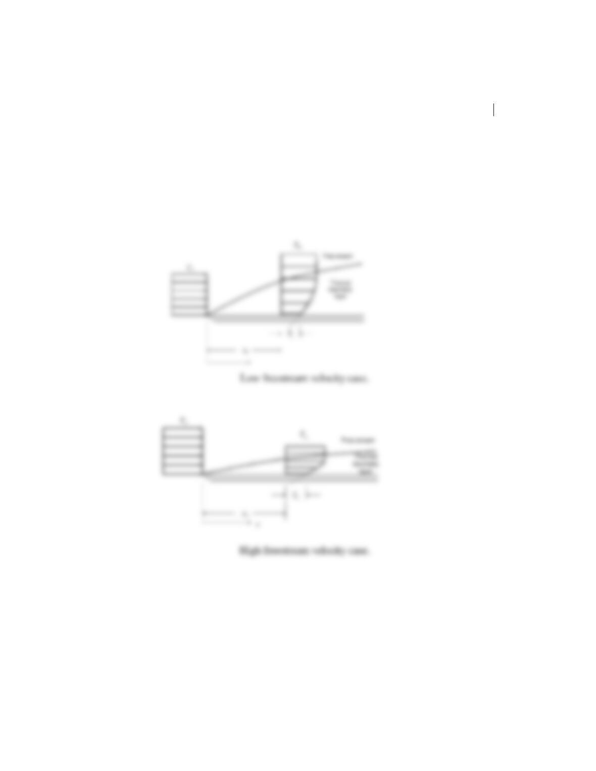
(b) At every location in the boundary layer, the temperature must vary from Ts at the surface to T∞ in

the free stream. This change must occur within the thermal boundary layer thickness, as shown in the

sketch below.

PROBLEM 6.1 (Cont.)

The magnitude of the heat flux is proportional to the temperature gradient at the surface,

0

/y

Ty

=

∂∂

,

which is shown schematically as a dashed line. The temperature gradient is steeper (larger) at x1

where the thermal boundary layer is thinner and less steep (smaller) at x3 where the thermal boundary

layer is thicker. Therefore, the magnitude of the local heat flux is largest at x1 and smallest at x3. <

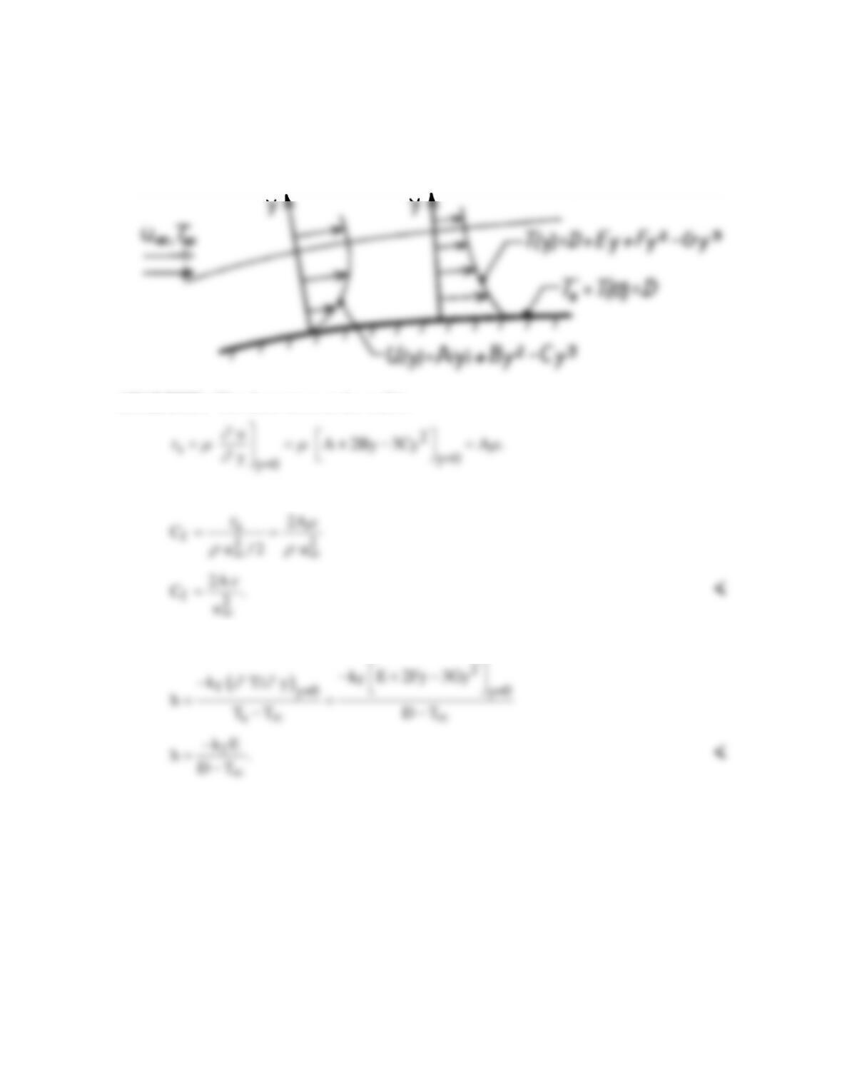
(c) As the free stream velocity increases the boundary layer becomes thinner. Sketches for a low and

high free stream velocity are shown below.

The temperature gradient, shown as the dashed line, is steeper for the higher free stream velocity case.

Therefore the higher free stream velocity case has the higher convective heat flux. <

COMMENTS: It is important to understand how the temperature gradient at the surface varies as the

thickness of the boundary layer changes.

PROBLEM 6.2

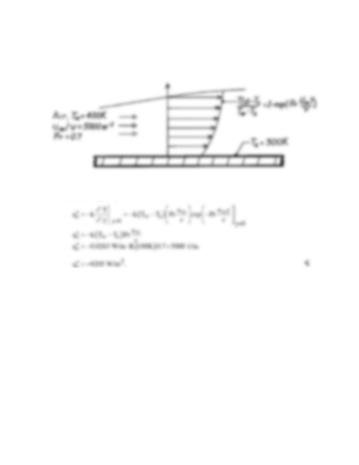
KNOWN: Form of the velocity and temperature profiles for flow over a surface.

FIND: Expressions for the friction and convection coefficients.

SCHEMATIC:

ANALYSIS: The shear stress at the wall is

Hence, the friction coefficient has the form,

The convection coefficient is

COMMENTS: It is a simple matter to obtain the important surface parameters from

knowledge of the corresponding boundary layer profiles. However, it is rarely a simple matter

to determine the form of the profile.

PROBLEM 6.3

KNOWN: Boundary layer temperature distribution.

FIND: Surface heat flux.

SCHEMATIC:

PROPERTIES: Table A-4, Air (Ts = 300K): k = 0.0263 W/m⋅K.

ANALYSIS: Applying Fourier’s law at y = 0, the heat flux is

COMMENTS: (1) Negative flux implies convection heat transfer to the surface.

(2) Note use of k at Ts to evaluate

s

q′′

from Fourier’s law.

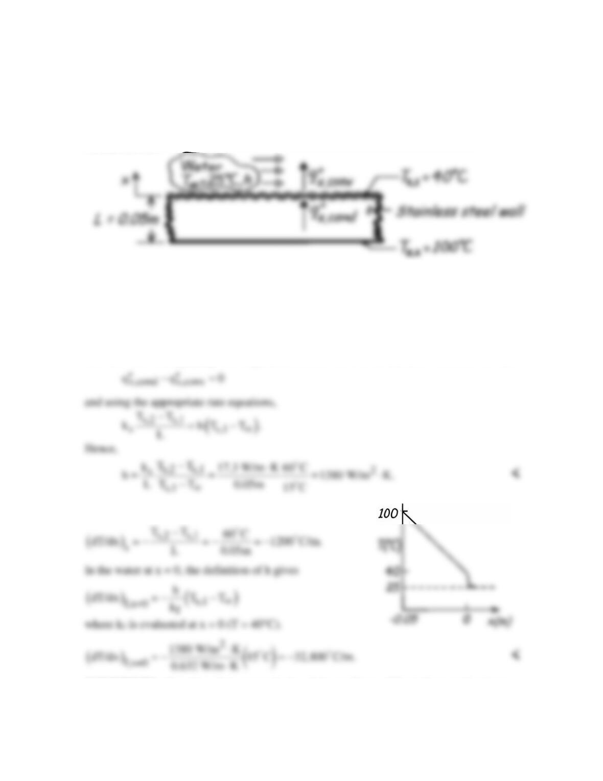
PROBLEM 6.4

KNOWN: Surface temperatures of a steel wall and temperature of water flowing over the

wall.

FIND: (a) Convection coefficient, (b) Temperature gradient in wall and in water at wall

surface.

SCHEMATIC:

ASSUMPTIONS: (1) Steady–state conditions, (2) One-dimensional heat transfer in x, (3)

Constant properties.

PROPERTIES: Table A-1, Stainless steel Type AISI 302 (70°C = 343K), ks = 17.3 W/m⋅K;

Table A-6, Water (40°C = 313 K), kf = 0.632 W/m⋅K.

ANALYSIS: (a) Applying an energy balance to the control surface at x = 0, it follows that

(b) The gradient in the wall at the surface is

COMMENTS: Note the relative magnitudes of the gradients. Why is there such a large

difference?

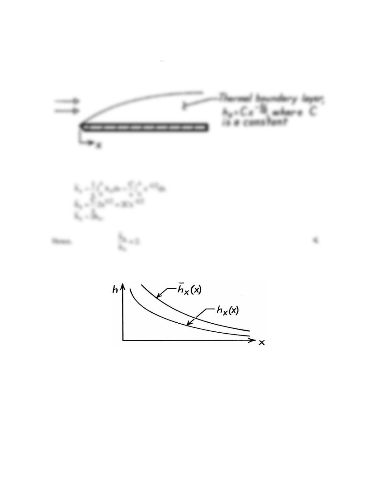
PROBLEM 6.5

KNOWN: Variation of hx with x for laminar flow over a flat plate.

FIND: Ratio of average coefficient,

x

h,

to local coefficient, hx, at x.

SCHEMATIC:

ANALYSIS: The average value of hx between 0 and x is

COMMENTS: Both the local and average coefficients decrease with increasing distance x

from the leading edge, as shown in the sketch below.

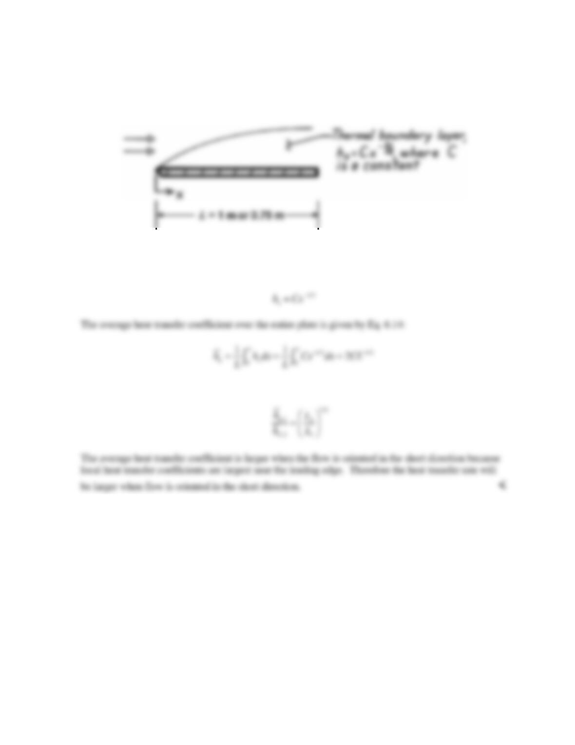
PROBLEM 6.6

KNOWN: Variation of local heat transfer coefficient with x. Length of plate.

FIND: Ratio of heat transfer coefficients for flow oriented in short and long directions.

SCHEMATIC:

ASSUMPTIONS: (1) Steady–state conditions, (2) Laminar flow, (3) Incompressible flow.

ANALYSIS: The local heat transfer coefficient varies with x according to

Therefore the ratio of average heat transfer coefficients for the two different flow orientations is

COMMENTS: Many engineering devices that are affected by, or utilize convection heat transfer in

their operation incorporate short sections of surfaces in order to take advantage of the high local heat

transfer coefficients that exist near the leading edges of such surfaces.

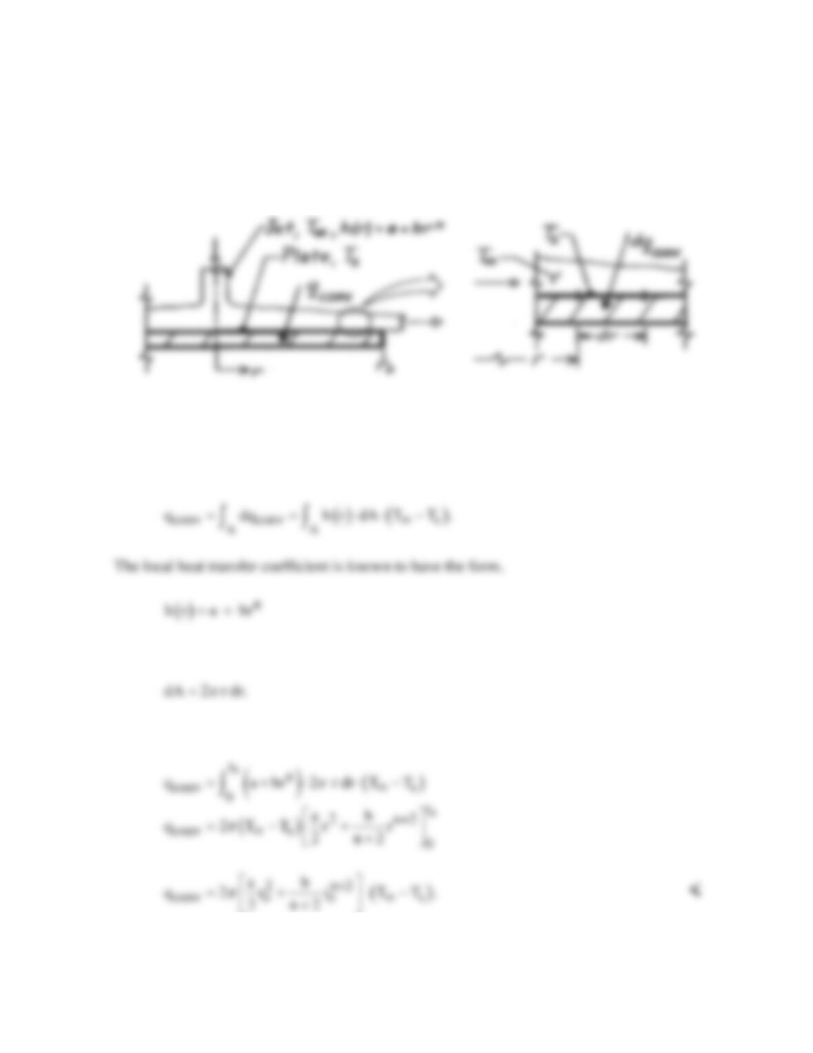
PROBLEM 6.7

KNOWN: Expression for the local heat transfer coefficient of a circular, hot gas jet at T∞

directed normal to a circular plate at Ts of radius ro.

FIND: Heat transfer rate to the plate by convection.

SCHEMATIC:

ASSUMPTIONS: (1) Steady-state conditions, (2) Flow is axisymmetric about the plate, (3)

For h(r), a and b are constants and n ≠ -2.

ANALYSIS: The convective heat transfer rate to the plate follows from Newton’s law of

cooling

and the differential area on the plate surface is

Hence, the heat rate is

COMMENTS: Note the importance of the requirement, n ≠ -2. Typically, the radius of the

jet is much smaller than that of the plate.

PROBLEM 6.8

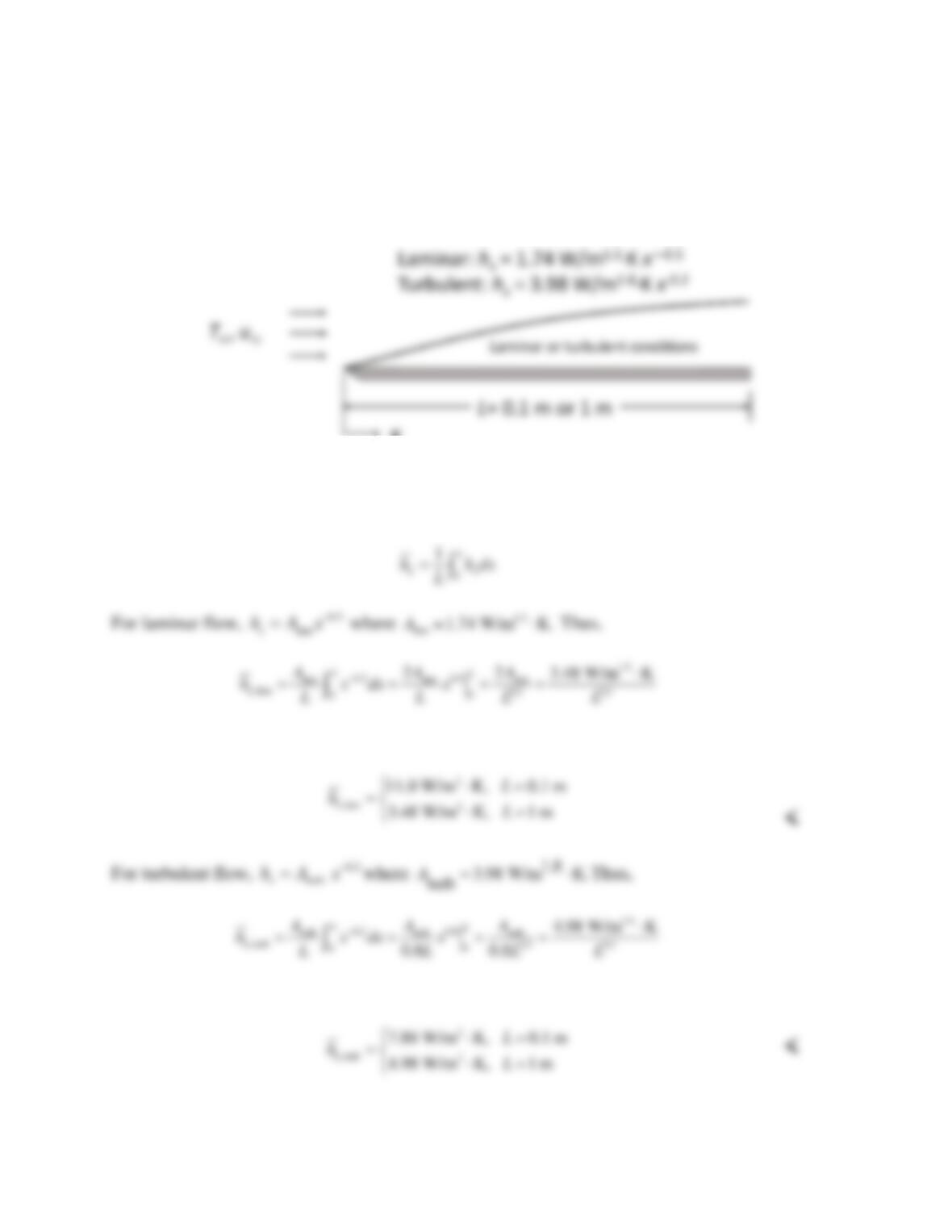
KNOWN: Smooth flat plate with either laminar or turbulent conditions starting at the leading edge.

Corresponding heat transfer coefficient correlations.

FIND: Average heat transfer coefficients for both conditions for plates of length L = 0.1 m and 1 m.

SCHEMATIC:

x

ASSUMPTIONS: (1) Steady–state conditions, (2) Two-dimensional flow and heat transfer.

ANALYSIS: The average heat transfer coefficient is defined as:

The results for the two plate lengths are:

COMMENTS: For L = 1 m, the turbulent heat transfer coefficient is larger than the laminar one, as is

usually the case. However, for L =0.1 m, the situation is reversed.

PROBLEM 6.9

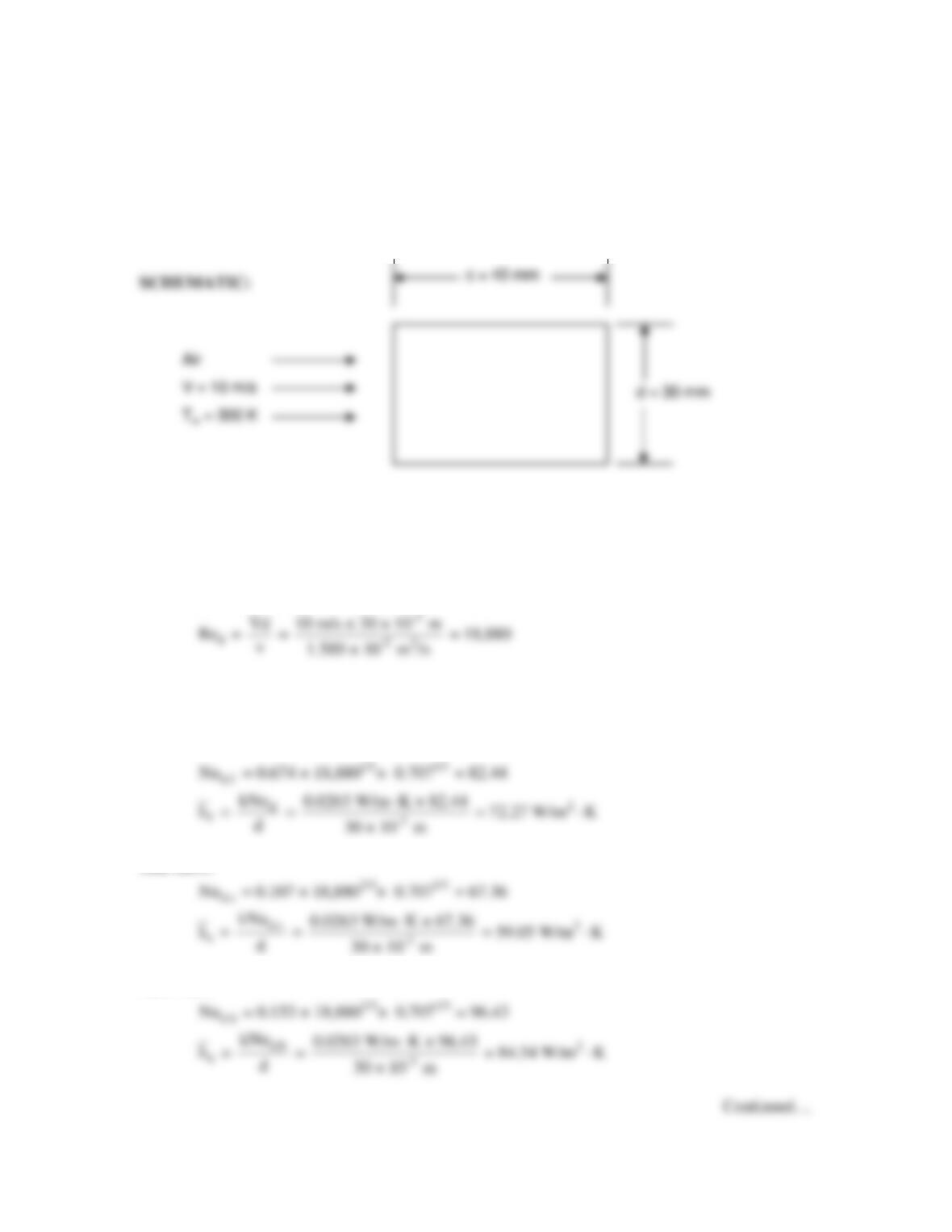
KNOWN: Expression for face–averaged Nusselt numbers on a cylinder of rectangular cross

section. Dimensions of the cylinder.

FIND: Average heat transfer coefficient over the entire cylinder. Plausible explanation for

variations in the face-averaged heat transfer coefficients.

ASSUMPTIONS: (1) Steady-state conditions, (2) Constant properties.

PROPERTIES: Table A.4, air (300 K): k = 0.0263 W/m⋅K, ν = 1.589 × 10-5 m2/s, Pr = 0.707.

ANALYSIS:

For the square cylinder, c/d = 40 mm/30 mm = 1.33

Therefore, for the front face C = 0.674, m = ½. For the sides, C = 0.107, m = 2/3 while for the

back C = 0.153, m = 2/3.

Front face:

Side faces:

Back face:

PROBLEM 6.9 (Cont.)

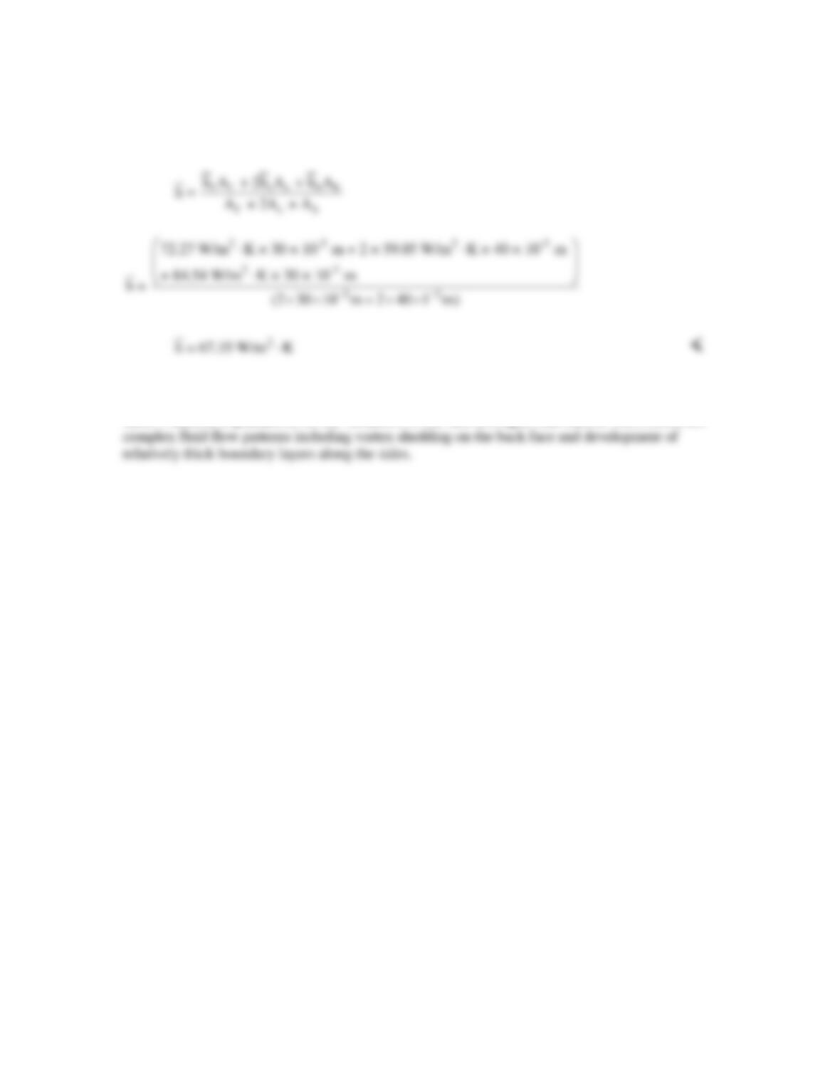
For the entire square cylinder of unit length,

The face–averaged heat transfer coefficients are largest on the back face and smallest on the side

faces. Plausible explanations for the variations of the face–averaged heat transfer coefficients are

COMMENT: See S.Y. Yoo, J.H. Park, C.H. Chung and M.K. Chung, Journal of Heat Transfer,

Vol. 125, pp. 1163-1169, 2003 for details.

PROBLEM 6.10

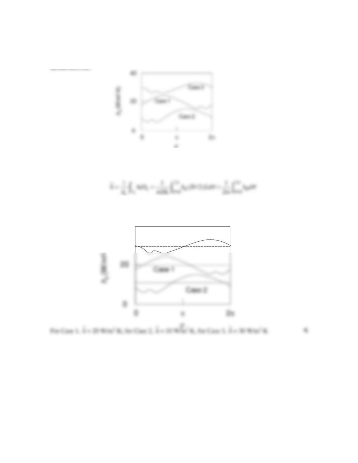
KNOWN: Variation of local heat transfer coefficient around a circular collector tube.

FIND: (a) Estimate the average heat transfer coefficient, (b) Case with highest collector efficiency.

ASSUMPTIONS: Solar irradiation is independent of the reflector orientation.

ANALYSIS: (a) From Eq. 6.13,

s

where L is the collector tube length. Hence, the average heat transfer coefficient may be estimated as

the average value of the local heat transfer coefficient. Approximate values of the average heat transfer

coefficient are shown in the sketch below.

(b) The collector tube will be hotter than the ambient air. Hence, convective losses from the collector

tube will diminish the overall collector efficiency. Therefore, Case 2 will have the highest collector

efficiency. <

COMMENTS: (1) For case 2, the parabolic reflector partially “shields” the collector tube from the

wind, resulting in reduced heat transfer coefficients. The flow adjacent to the tube also experiences a

change in direction for case 2, with a large recirculation pattern established behind the reflector. (2)

None of the cases experiences symmetrical flow over the collector tube, as would be expected without

the reflector in place. (3) See Naeeni and Yaghoubi, “Analysis of Wind Flow Around a Parabolic

Collector (2) Heat Transfer from Receiver Tube,” Renewable Energy, Vol. 32, pp. 1259 – 1272, 2007,

for additional discussion.

θ

40

Case 3

PROBLEM 6.11

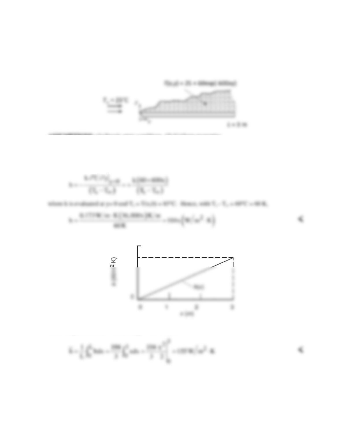
KNOWN: Temperature distribution in boundary layer for helium flow over a flat plate.

FIND: Variation of local convection coefficient along the plate and value of average coefficient.

SCHEMATIC:

ASSUMPTIONS: (1) Steady-state conditions, (2) Uniform properties.

PROPERTIES: Table A-4, Helium (Ts = 85°C = 358 K), k = 0.173 W/m⋅K.

ANALYSIS: From Eq. 6.5,

and the convection coefficient increases linearly with x.

350

311

The average coefficient over the range 0 ≤ x ≤ 3 m is

PROBLEM 6.12

KNOWN: Variation of local convection coefficient with distance x from a heated plate with a

uniform temperature Ts.

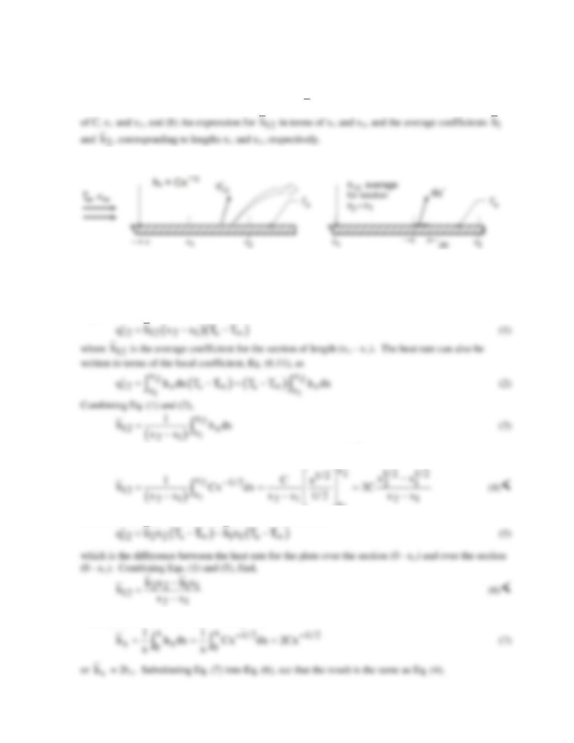
FIND: (a) An expression for the average coefficient

12

h

for the section of length (x2 – x1) in terms

SCHEMATIC:

ASSUMPTIONS: (1) Laminar flow over a plate with uniform surface temperature, Ts, and (2)

Spatial variation of local coefficient is of the form

1/ 2

x

h Cx

−

=

, where C is a constant.

ANALYSIS: (a) The heat transfer rate per unit width from a longitudinal section, x2 – x1, can be

expressed as

12

h

and substituting for the form of the local coefficient,

1/ 2

x

h Cx

−

=

, find that

1

x

(b) The heat rate, given as Eq. (1), can also be expressed as

COMMENTS: (1) Note that, from Eq. 6.6,

12

h

PROBLEM 6.13

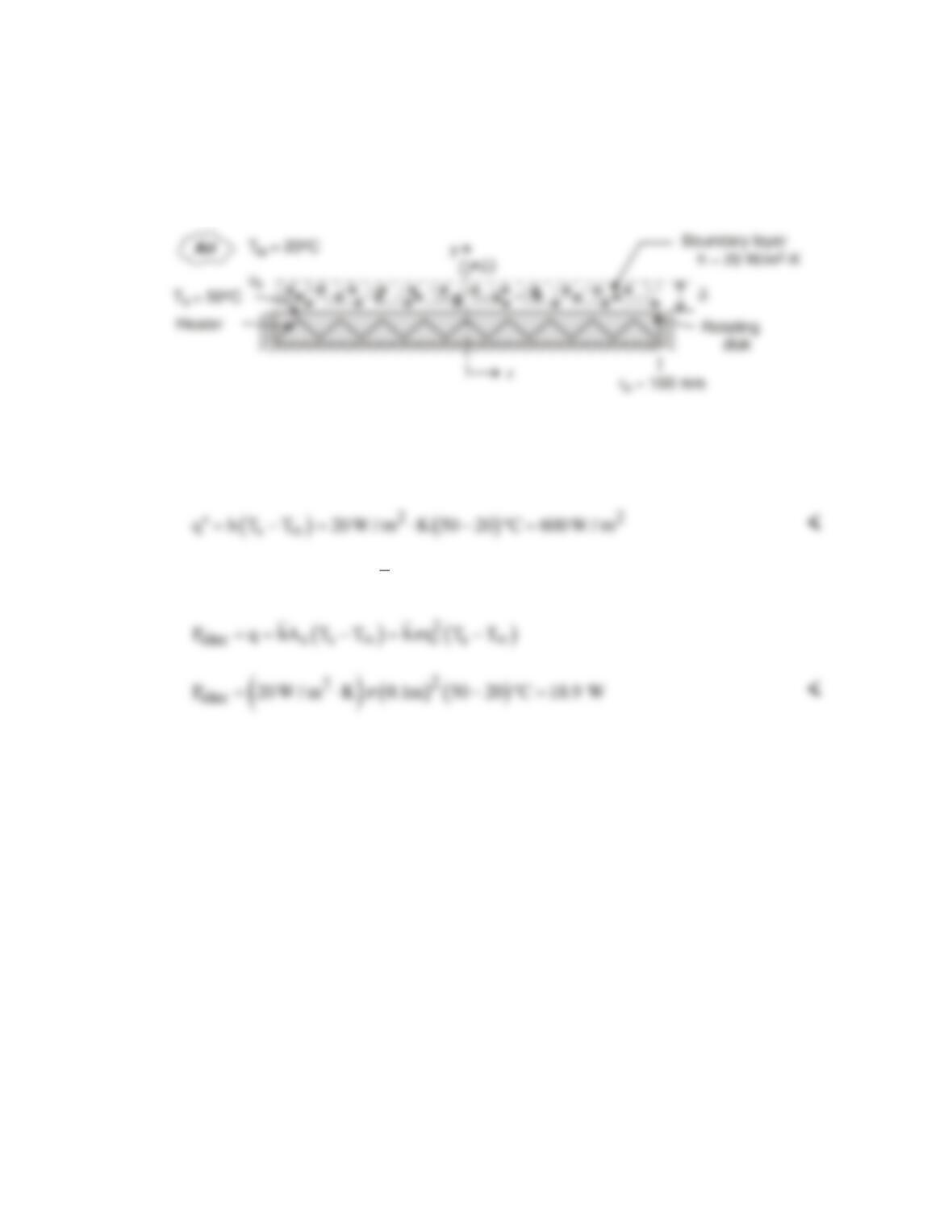
KNOWN: Local convection coefficient on rotating disk. Radius and surface temperature of disk.

Temperature of stagnant air.

FIND: Local heat flux and total heat rate. Nature of boundary layer.

SCHEMATIC:

ASSUMPTIONS: (1) Negligible heat transfer from back surface and edge of disk.

ANALYSIS: If the local convection coefficient is independent of radius, the local heat flux at every

point on the disk is

Since h is independent of location,

2

h h 20 W / m K= = ⋅

and the total power requirement is

If the convection coefficient is independent of radius, the boundary layer must be of uniform

thickness d. Within the boundary layer, air flow is principally in the circumferential direction. The

circumferential velocity component uθ corresponds to the rotational velocity of the disk at the surface

(y = 0) and increases with increasing r (uθ = Ωr). The velocity decreases with increasing distance y

from the surface, approaching zero at the outer edge of the boundary layer (y → d).

PROBLEM 6.14

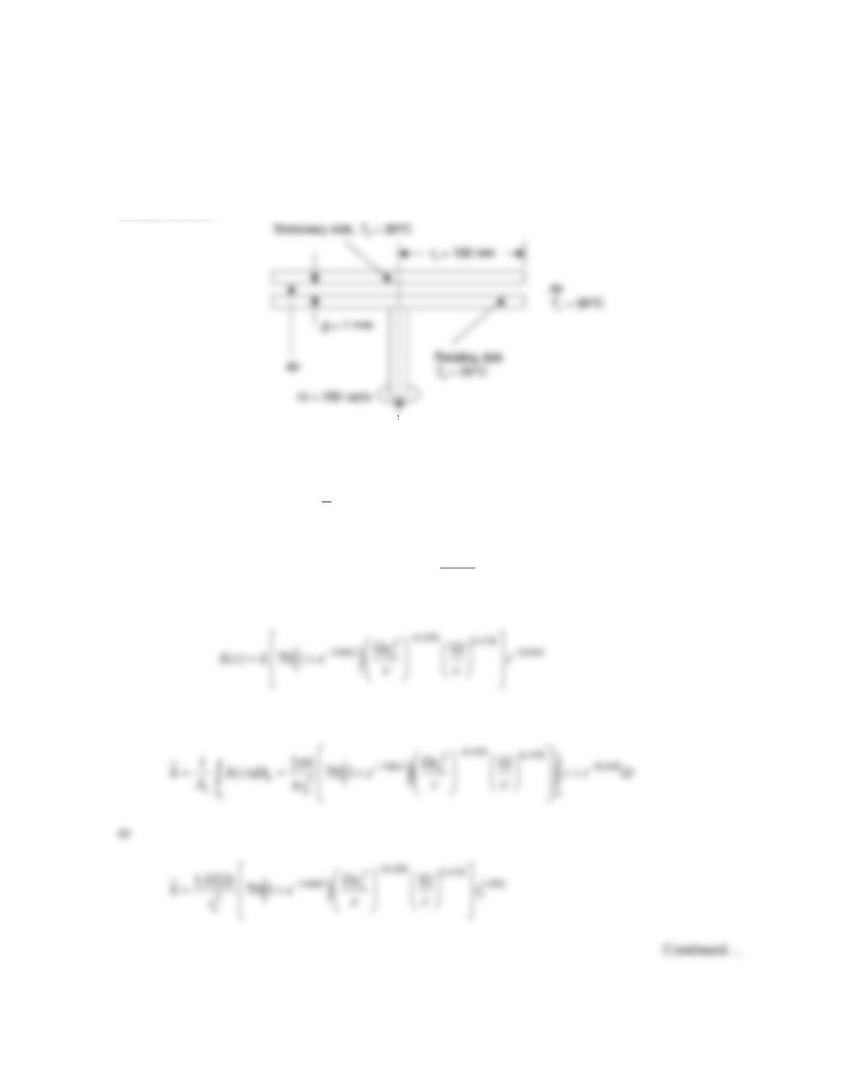
KNOWN: Dimensions and temperatures of rotating and stationary disks, air gap spacing between

disks, rotational speed. Correlation for the local Nusselt number.

FIND: Value of the average Nusselt number, total heat flux from the disk’s top surface, total power

requirement. Comment on the nature of the flow between the disks.

SCHEMATIC:

ASSUMPTIONS: (1) Steady–state conditions, (2) Constant properties, (3) Negligible viscous

dissipation.

PROPERTIES: Table A-4, air (

T

= (50°C + 20°C)/2 = 35°C ≈ 308K):

ν

= 16.69×10-6 m2/s, k =

0.0269 W/m⋅K.

ANALYSIS: From the problem statement,

( )

140 0.456 0.478

() 70 1

o

G

r rr

hrr

Nu e Re Re

k

−−

= = +

.

Since

2/

r

Re r

ν

= Ω

, the local heat transfer coefficient is

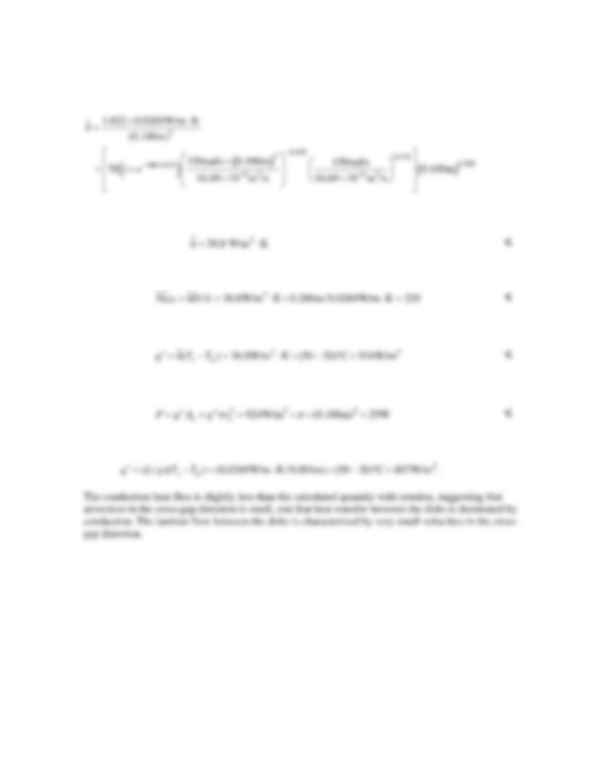
The average heat transfer coefficient may be evaluated from

PROBLEM 6.14 (Cont.)

Substituting values,

or

The average Nusselt number is

The heat flux from the top surface of the disk is

Therefore, the total electric power requirement is

Note that if only conduction were occurring between the two disks, the heat flux would be

COMMENTS: (1) The slight increase in heat transfer rate is due to edge effects where air can exit

or enter the space between the disks, and enhance heat transfer between the disks by mixing. (2) The

Reynolds number is

( )

2

2 62

/ 150rad/s 0.100m /16.69 10 m / s 90,000.

o

ro

Re r

ν

−

=Ω= × × =

Transition to

turbulent flow begins at a Reynolds number of approximately 180,000 for this configuration. (3) See

Pelle and Harmand, “Heat Transfer Measurements in an Opened Rotor–Stator System Air–Gap,”

Experimental Thermal and Fluid Science, ‘Vol. 31, pp. 165 – 180, 2007, for more information.

PROBLEM 6.15

KNOWN: Air flow over a flat plate of known length, location of transition from laminar to

turbulent flow, value of the critical Reynolds number.

FIND: (a) Free stream velocity with properties evaluated at T = 350 K, (b) Expression for the

average convection coefficient,

lam

h (x)

, as a function of the distance x from the leading edge in

the laminar region, (c) Expression for the average convection coefficient

turb

h (x)

, as a function

of the distance x from the leading edge in the turbulent region, (d) Compute and plot the local and

average convection coefficients over the entire plate length.

SCHEMATIC:

ASSUMPTIONS: (1) Steady-state conditions, (2) Constant properties.

PROPERTIES: Table A.4, air (T = 350 K): k = 0.030 W/m⋅K, ν = 20.92 × 10-6 m2/s, Pr = 0.700.

ANALYSIS:

(a) Using air properties evaluated at 350 K with xc = 0.5 m,

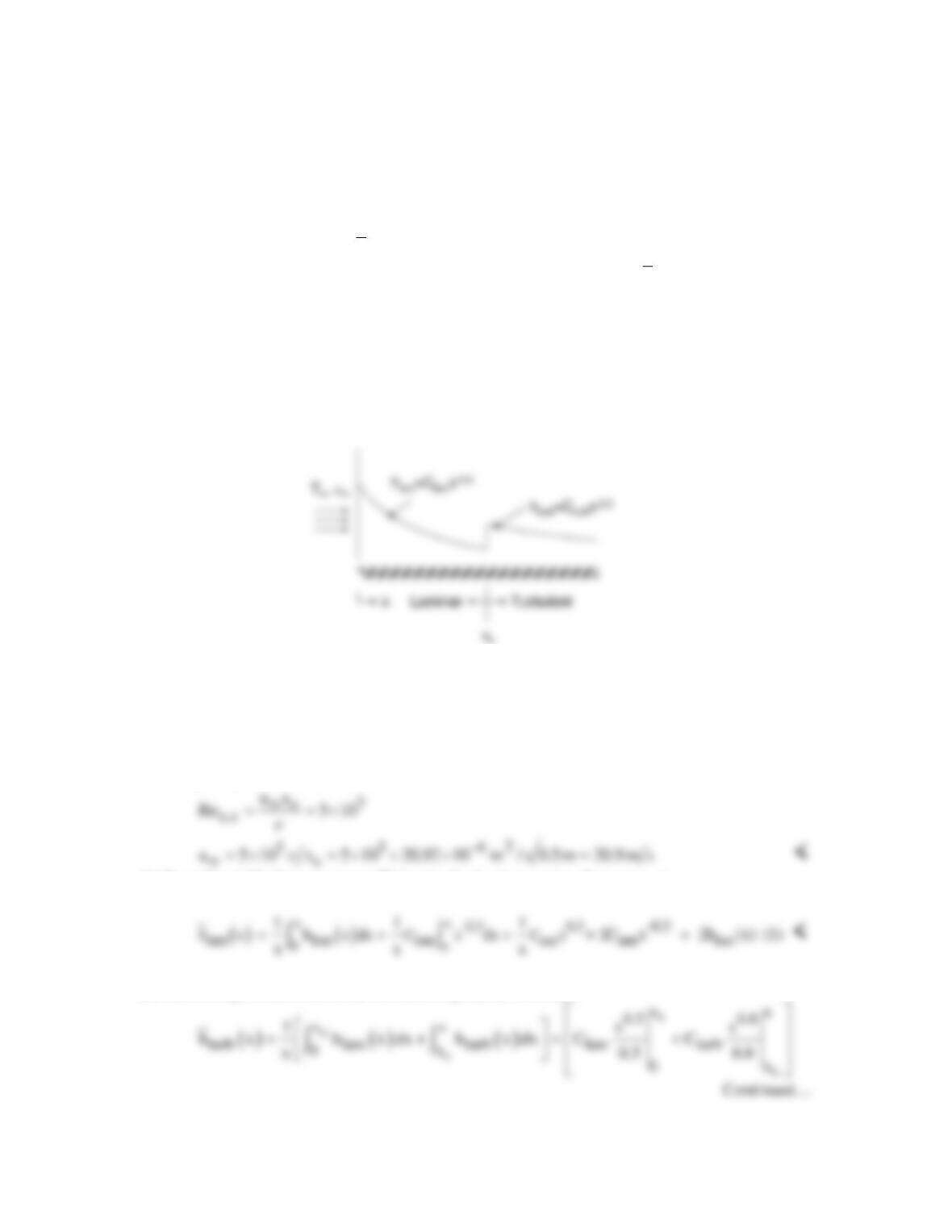
(b) From Eq. 6.13, the average coefficient in the laminar region, 0 ≤ x ≤ xc, is

(c) The average coefficient in the turbulent region, xc ≤ x ≤ L, is

PROBLEM 6.15 (Cont.)

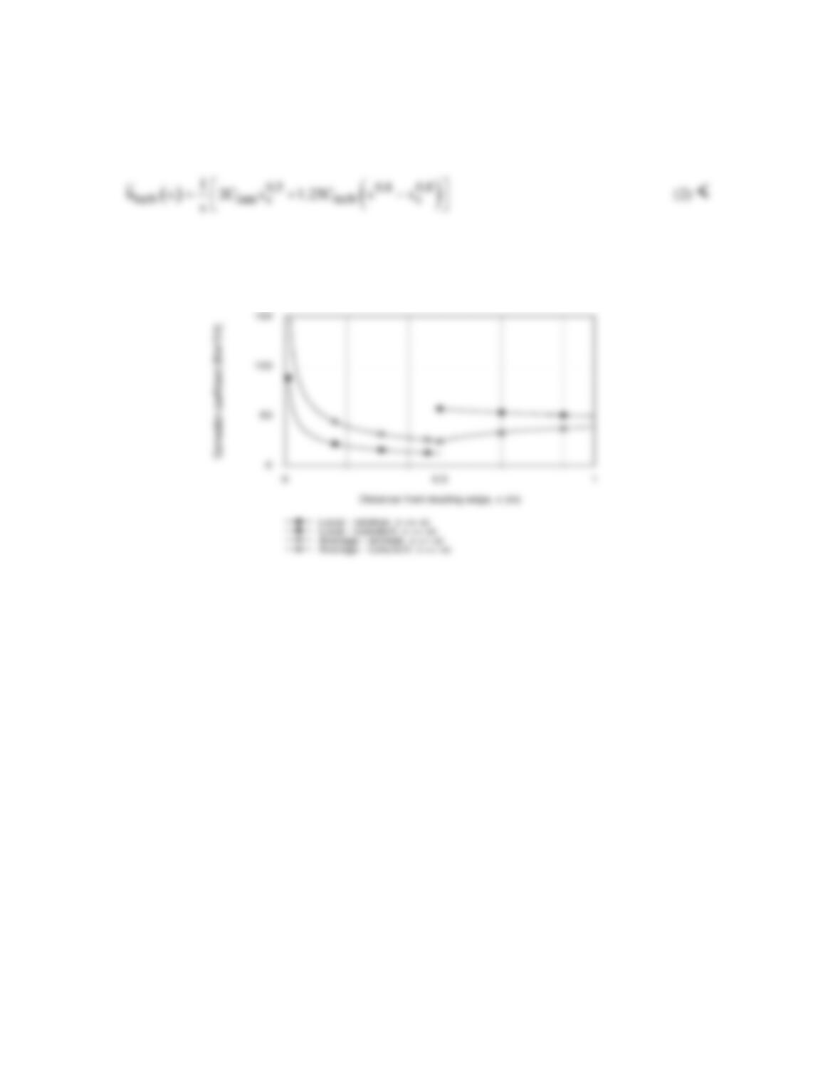
(d) The local and average coefficients, Eqs. (1) and (2) are plotted below as a function of x for the

range 0 ≤ x ≤ L.

PROBLEM 6.16

KNOWN: Air speed and temperature in a wind tunnel.

FIND: (a) Minimum plate length to achieve a Reynolds number of 107, (b) Distance from

leading edge at which transition would occur.

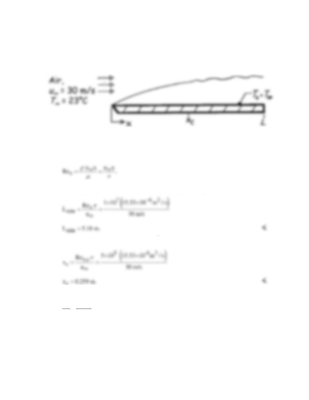
SCHEMATIC:

ASSUMPTIONS: (1) Isothermal conditions, Ts = T∞.

PROPERTIES: Table A-4, Air (23°C = 296K): ν = 15.53 × 10-6m2/s.

ANALYSIS: (a) The Reynolds number is

To achieve a Reynolds number of 1 × 107, the minimum plate length is then

(b) For a transition Reynolds number of 5 × 105

c

COMMENTS: Note that

x,c

c

L

Re

x

L Re

=

This expression may be used to quickly establish the location of transition from knowledge of

Re .

x,c L

and Re