1
ANSWERS TO CHAPTER 6 QUESTIONS
ANSWER 6.1
The NPV equation should be used to evaluate these two proposals:
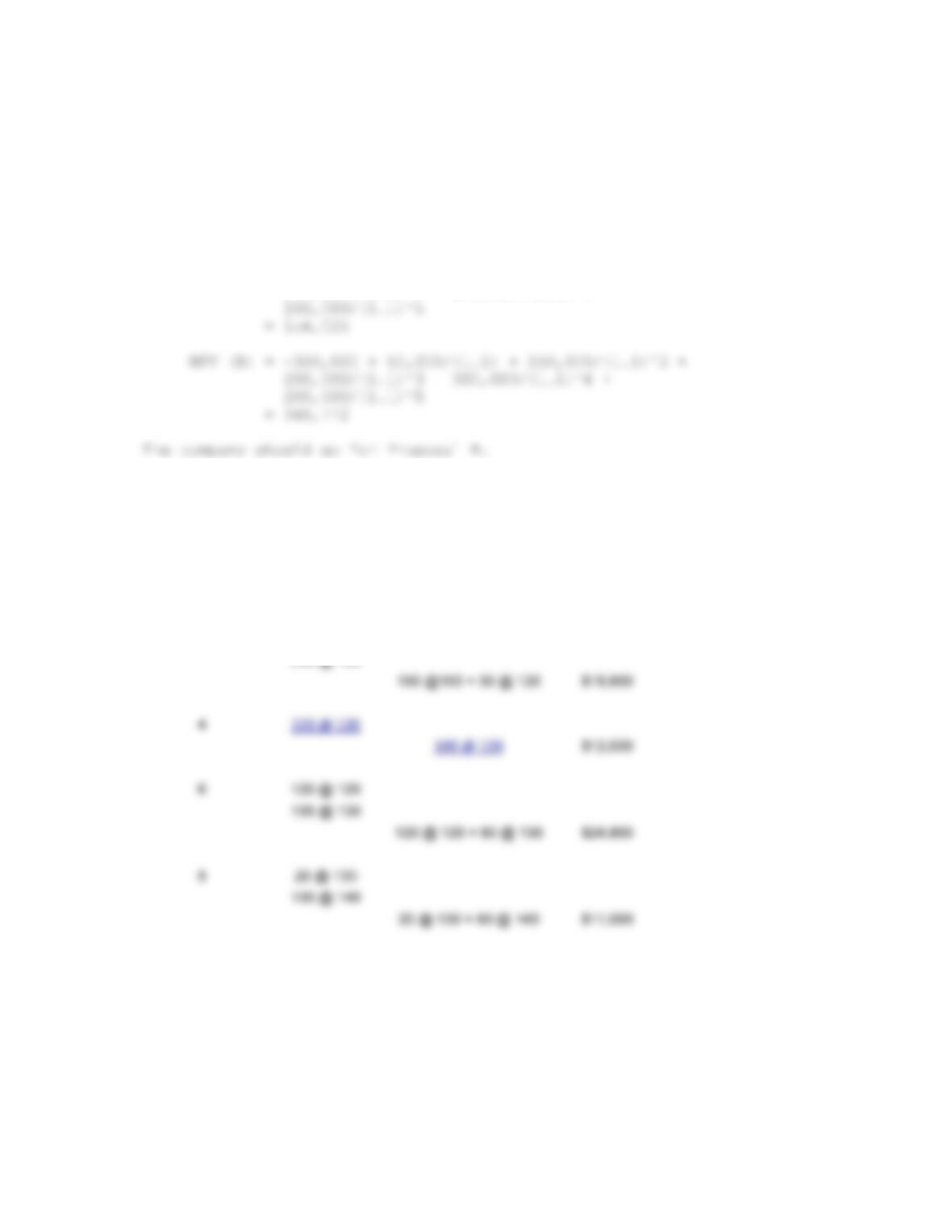
NPV (A) = -500,000 + 150,000/(1.1) + 200,000/(1.1)^2 +
250,000/(1.1)^3 + 150,000/(1.1)^4 +
ANSWER 6.2
The stock prices for FIFO withdrawal are shown in Table 6.27:
TABLE 6.27 FIFO WITHDRAWAL
Period Inventory FIFO Withdrawal Value
3 150 @ 100
250 @ 120
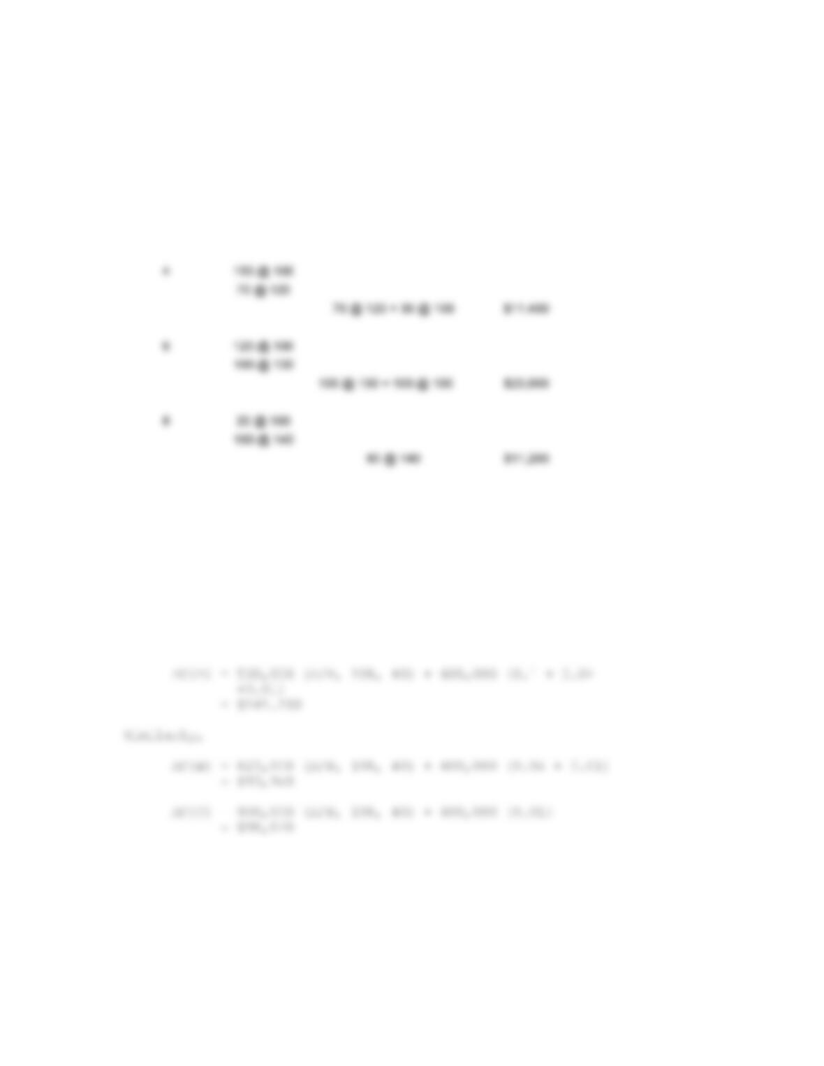
Similarly, the stock prices for LIFO withdrawal are shown in Table
6.28:
2
TABLE 6.28 LIFO WITHDRAWAL
Period Inventory LIFO Withdrawal Value
3 150 @ 100
250 @ 120
180 @ 120 $21,600
ANSWER 6.3
The sum of the construction cost and the expected damage needs to
be minimized.
If alternative A is chosen, it will have a capacity of 1 unit. Its
capacity will be exceeded (causing $600,000 damage) when the annual
rainfall exceeds 1 unit. The probability of the rainfall to exceed 1
unit is 0.15 (= 0.1 + 0.04 + 0.01). Hence, with no maintenance and
zero salvage value, the Annual Cost for the Alternative A is:
Alternative B should be chosen.
ANSWER 6.4
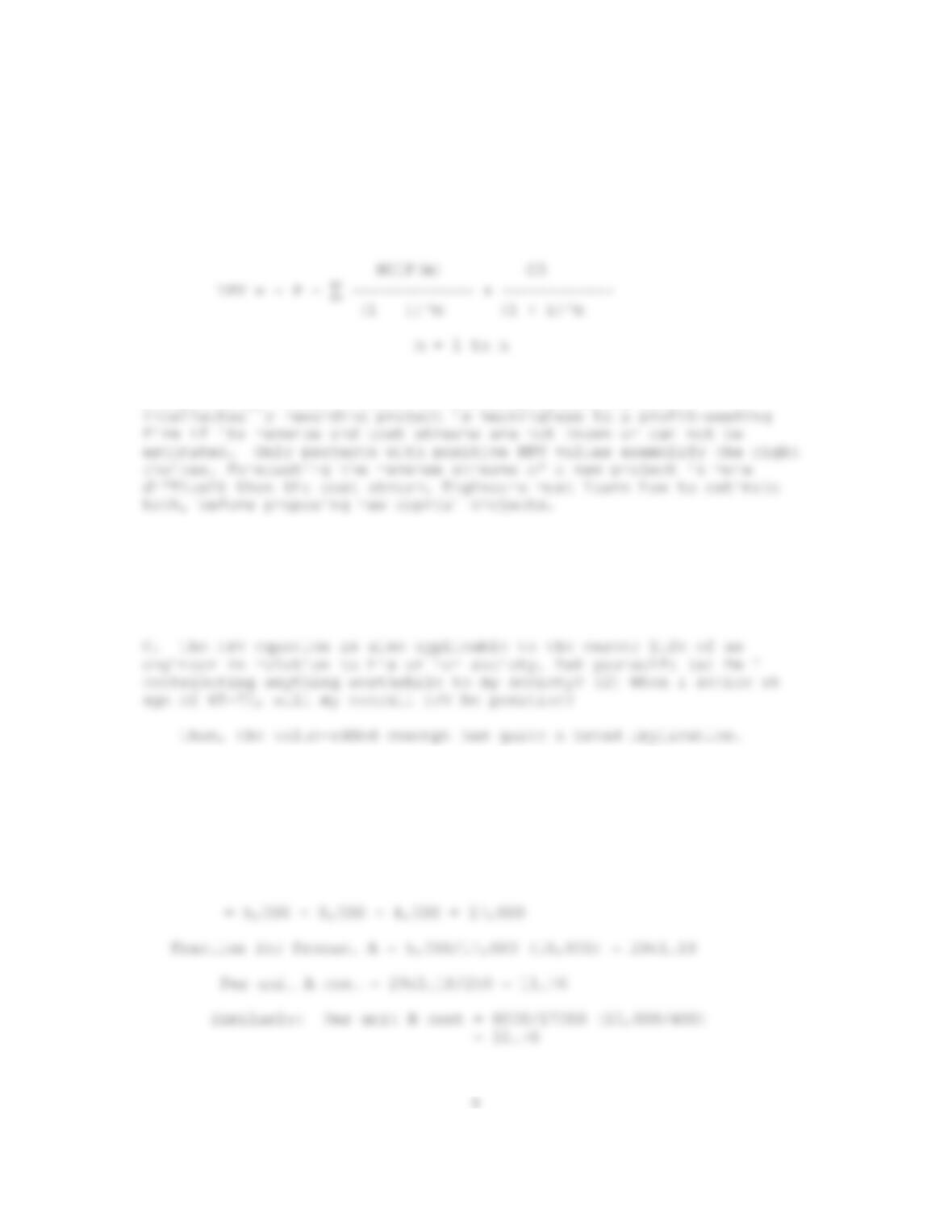
The Net Present Value Equation focuses on calculating NPV, the net
value added in present dollars of an investment project (e.g., R&D
project, capital project, etc.). Several important points may be
derived from this equation:
A. For a project to be worth pursuing, one must know the Net Cash In-
Flow, NCIF(m) = R(m) C(m). A technically exciting and
B. The NPV equation also applies to the overall employment situation
of an engineer in a profit-seeking firm. Each engineer must constantly
ask himself/herself: (a) Have I added any value to my firm lately? (b)
Is my NPV to my firm positive? (c) Which are the things I should focus
on to add more value to my firm?
ANSWER 6.5
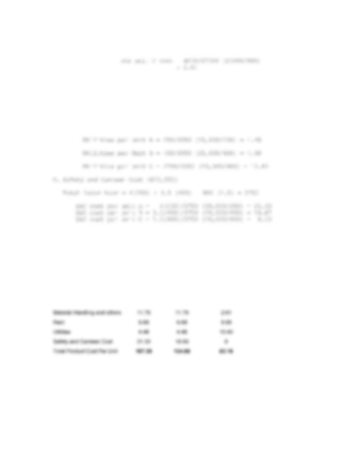
Applying Activity Based Costing yields the following:
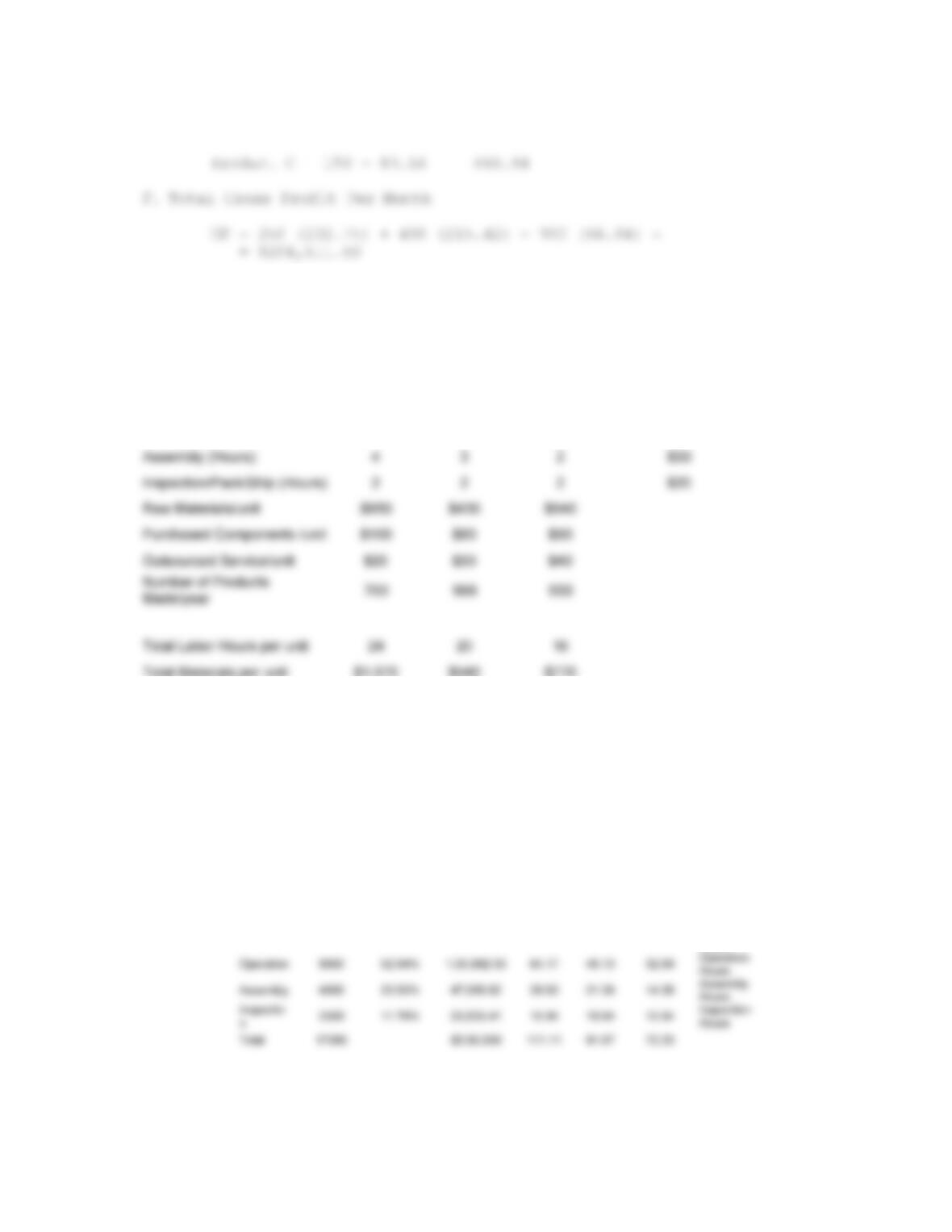
A. Material handling, waste and procurement ($10,000)
Total material costs of three products
4
B. Rent and Utilities ($30,000)
Assume that rent is 15,000 and utilities are 15,000.
(a) Rent per product = 15,000/(250+400+900) = 9.68 per unit
(b) Total machine hours = 250 (1) + 400 (1) + 900 (3) =
3350 hours
D. Compilation of Product Costs
The product costs are compiled in Table 6.29.
TABLE 6.29. PRODUCT COSTS
Product A Product B Product C
Material Cost 20 20 4.44
Labor Cost 100 70 45
E. Gross Profits for Products
Product A = 400 167.25 = $232.75
Product B = 350 134.58 = $215.42
5
ANSWER 6.6
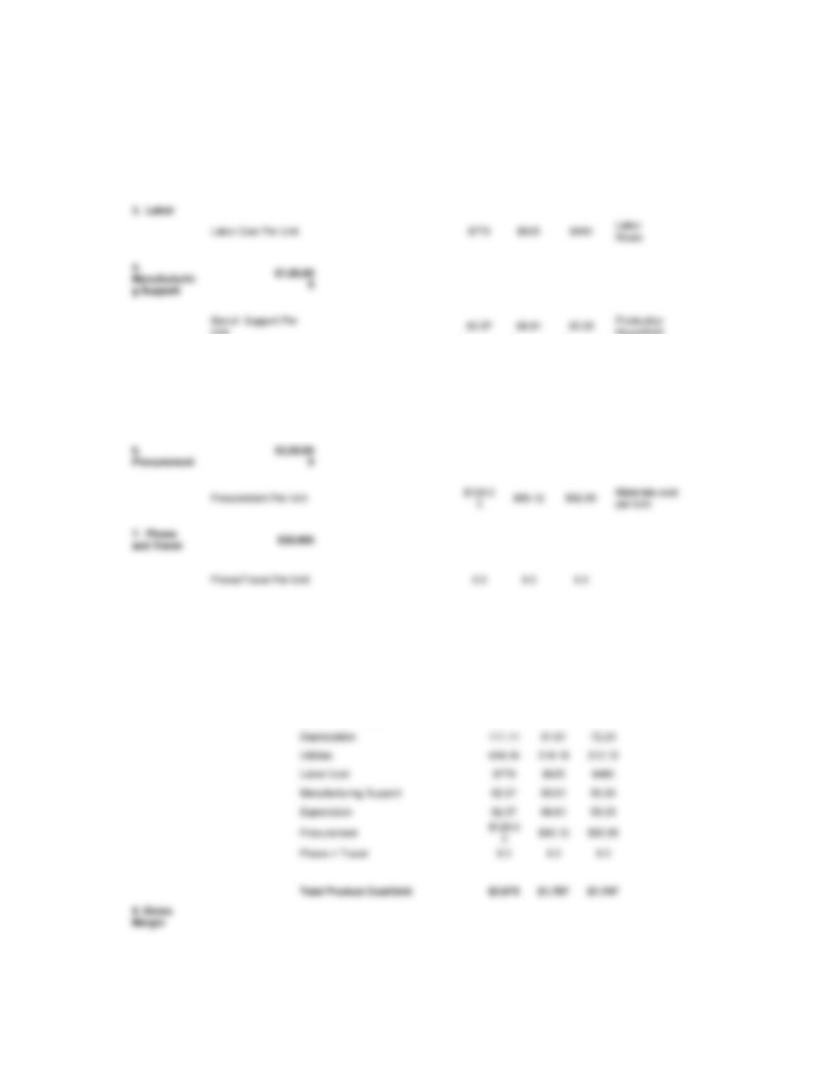
Table 6.30 lists the data given in this problem.
TABLE 6.30 OPERATIONS DATA FOR ALL PRODUCTS
Product A Product B Product C Labor Rate/hour
Machine Setup (Hours) 2 3 4 $25
Machine Operation (Hours) 16 12 8 $35
Table 6.31 which is shown on the next page illustrates how
product costs are computed using the Activity Based Costing method.
Table 6.31 ABC Analysis of Problem 6.6
1.
Depreciation
$2,00,00
0
Area Percentag
e
Depreciatio
n fraction
Produc
t A
Produc
t B
Product
C
Basis of
Cost
Allocation
Setup 2000 11.76% 23,529.41 7.47 11.2 14.94 Setup
Hours
6
2. Utilities $7,00,00
0
Utilities Per Unit 424.24 318.18 212.12 Operating
hours
Unit 82.57 68.81 55.05 Production
Hours/Unit
Produc
t A
Produc
t B
Product
C
5.
Supervision
$1,50,00
0
Supervision Per Unit 82.57 68.81 55.05 Production
Hours/Unit
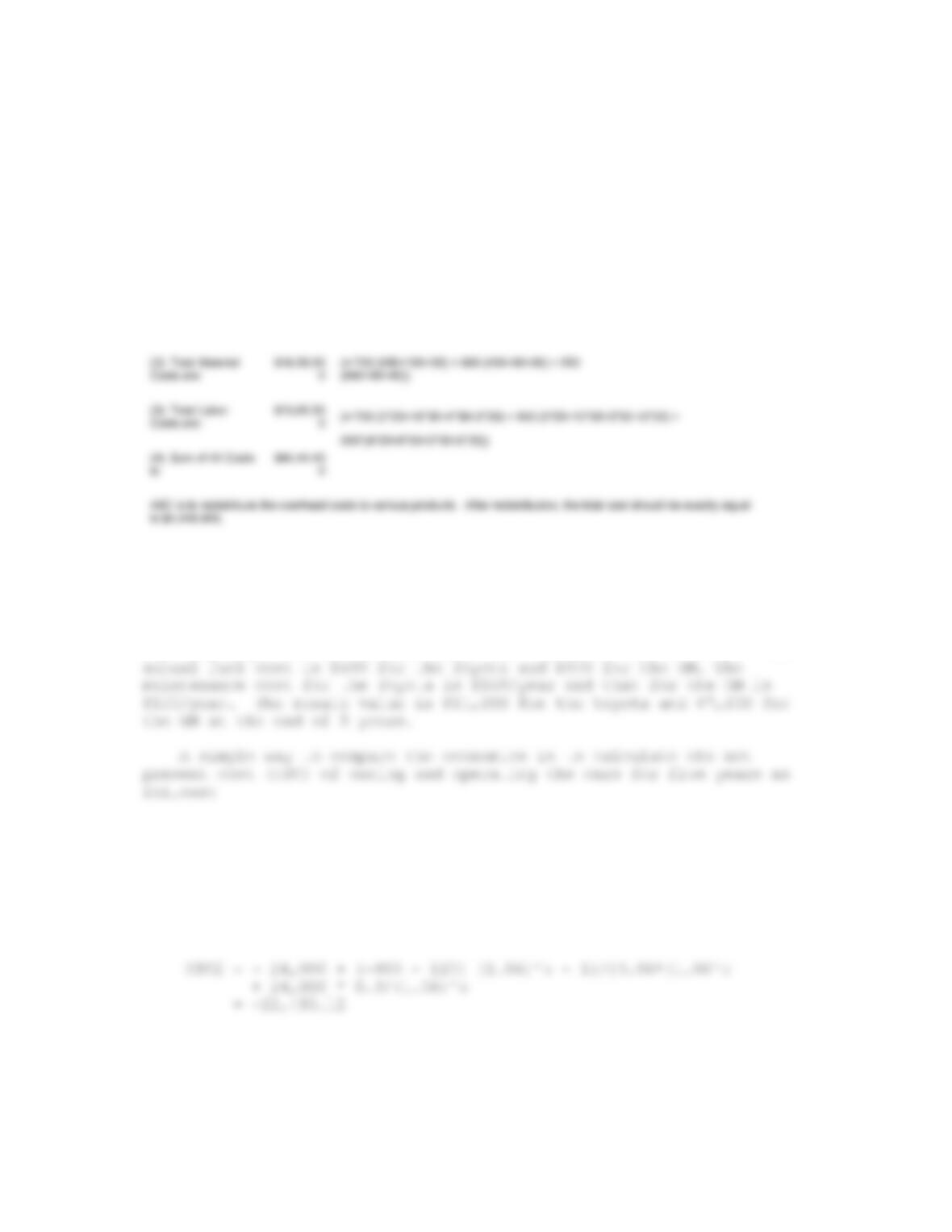
8. Summary of
Unit Product Cost
Produc
t A
Produc
t B
Produc
t C
Unit Product Cost Raw Materials $950 $430 $640
Purchased Components $100 $80 $90
Outsourced Service $20 $30 $40
7
Price/Unit $5,000 $4,500 $4,100
Gross Margin $2,321 $2,713 $2,353
Gross Margin % 46.42% 60.29% 57.40%
Total Gross Margin
Note: Strategic decision may be made in favor of Product B, which has the high gross margin percentage.
Note the comments:
(1) Total Overhead
Costs are:
$14,20,00
0(= 200,000 + 700,000 + 20,000 + 150,000 + 200,000 + 150,000)
ANSWER 6.7
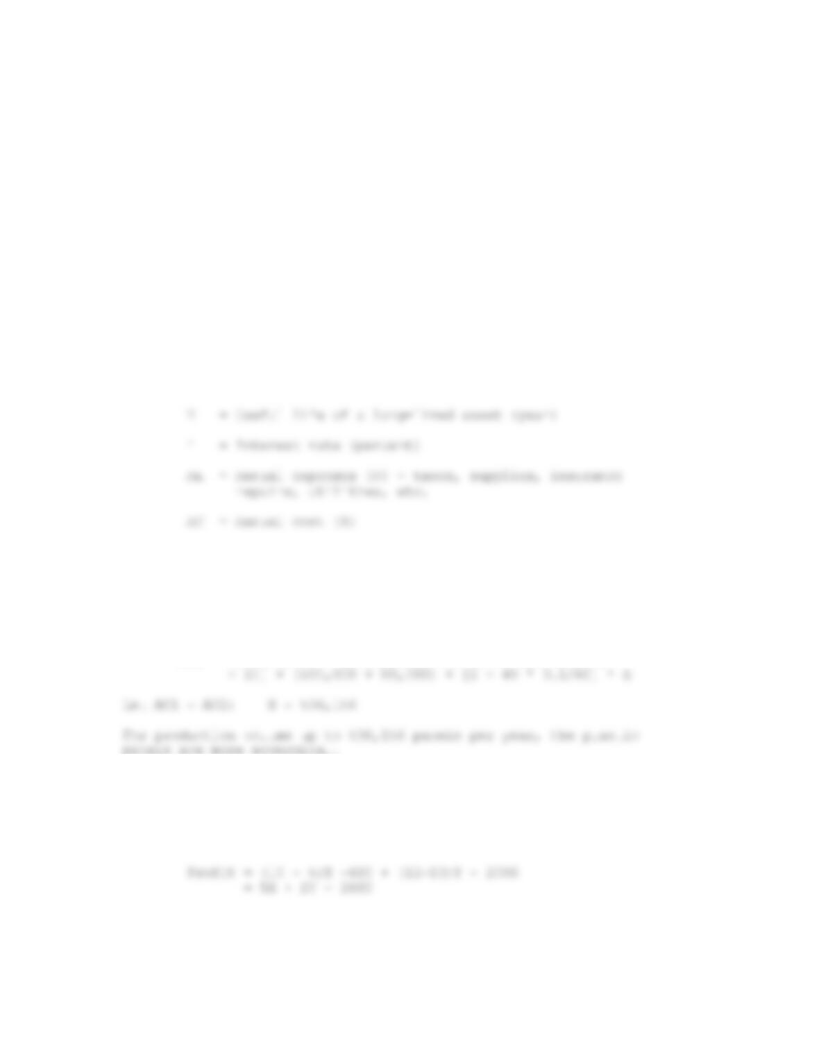
Compared to the GM, the Toyota is higher in price, lower in fuel
expense, higher in maintenance cost, and higher in resale value. The
A. Toyota
NPC1 = – 28,000 + (-400 140)[(1.06)^5 1]/[0.06
*(1.06)^5] + 28,000 * 0.4/(1.06)^5
= -21,905.38
B. GM
8
The above analysis points out that the total cost of owning and
operating the Toyota is less than that for the GM. The Toyota car is
to be preferred from the standpoint of costs.
ANSWER 6.8
This problem can be solved using the annual cost equation
(Equation 6.12).
(P L)* i
AC = —————– + P*i + AE (6.12)
[(1 + i)^N 1]
wherein:
P = Initial Investment ($)
L = Salvage Value ($)
Assume X = annual production volume, for plastic panels:
AC1 = (3,000,000 + 1,000,000)[0.06 (1.06)^10/(1.06^10
1)] + (500,000 + 100,000) + [5 + 40 * 2/60]* X
For steel panels:
AC2 = (25,000,000 + 4,000,000)[0.06 (1.06^15)/(1.06^15
panels are more economical.
ANSWER 6.9
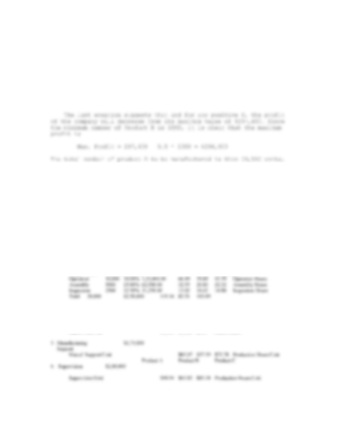
Let X and Y be the number of products A and B, respectively, to be
produced during a three-month period. The equation for calculating the
total profit is then:
9
On the other hand, the constraint imposed by the machining hours
states that:
30,000 = 0.5 X + 0.25 Y
Substituting X in the Profit equation, we have:
Profit = 5 (60,000 0.5 Y) + 2Y 2600 = 297,400 0.5 Y
ANSWER 6.10
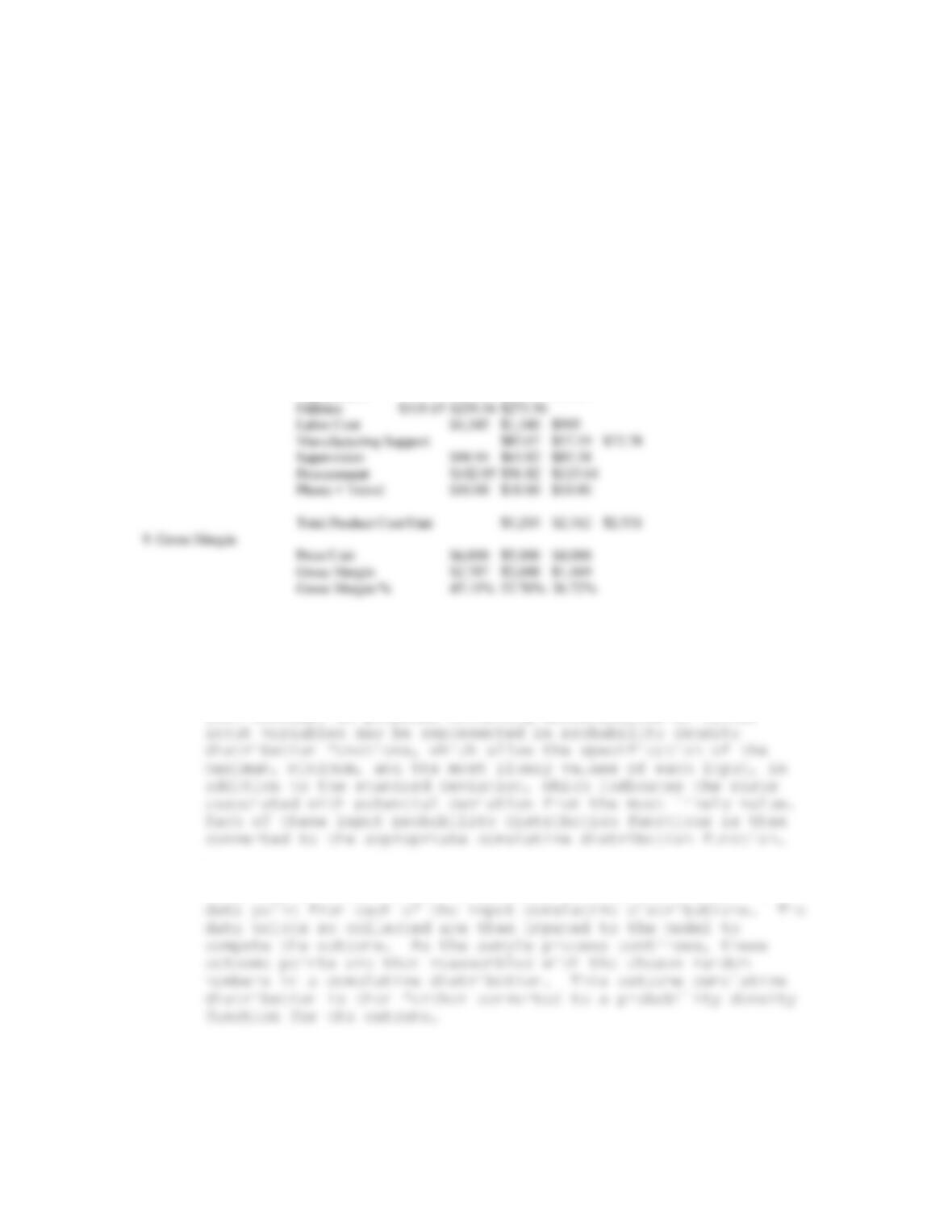
Detailed analyses are shown in Table 6.32. .
Table 6.32 ABC Solutions to Buffalo Best Company Problems
Product A Product B Product C
1. # of Products 800 1000 700
2. Depreciation $2,50,000
Area Percentage Depreciation Product A Product B Product C
Basis of Cost
Fraction Allocation
Setup 2500 12.50% 31,250.00 7.1 11.36 20.29 Setup Hours
3. Utilities $7,50,000
Utilities/Unit $319.15 $239.36 $273.56 Operating hours
4. Labor
Labor Cost/Unit $1,345 $1,140 $995 Labor Hours
10
7. Procurement $2,50,000
Procurement/Unit $142.05 $56.82 $113.64 Materials cost per Unit
8. Phone and Travel $25,000
Phone & Travel/Unit $10.00 $10.00 $10.00
9. Summary Product A Product B Product C
Unit Product Cost Raw Materials $1,000 $500 $700
Purchased Parts $150 $120 $130
Purchased Service $30 $40 $50
Depreciation 119.16 82.51 103.09
ANSWER 6.11
A. When addressing a cost problem of any kind, we usually set up a
mathematical cost model to link the input cost variables to the
cost outcome. In problems involving uncertainties or risks,
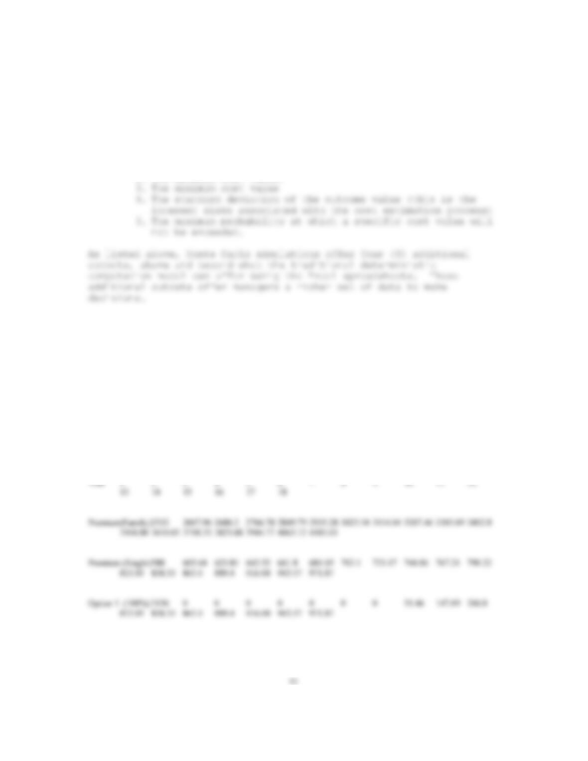
B. When the Monte Carlo simulations are activated to initiate a
sampling, a random number is selected to read off a specific
C. Because the cost outcome is produced in the form of probability
distribution function, it
contains five (5) specific results:
1. The Most likely cost outcome value (this is of course
equivalent to the outcome, when only the most like input
values are used in the cost model)
2. The maximum cost value.
ANSWER 6.12
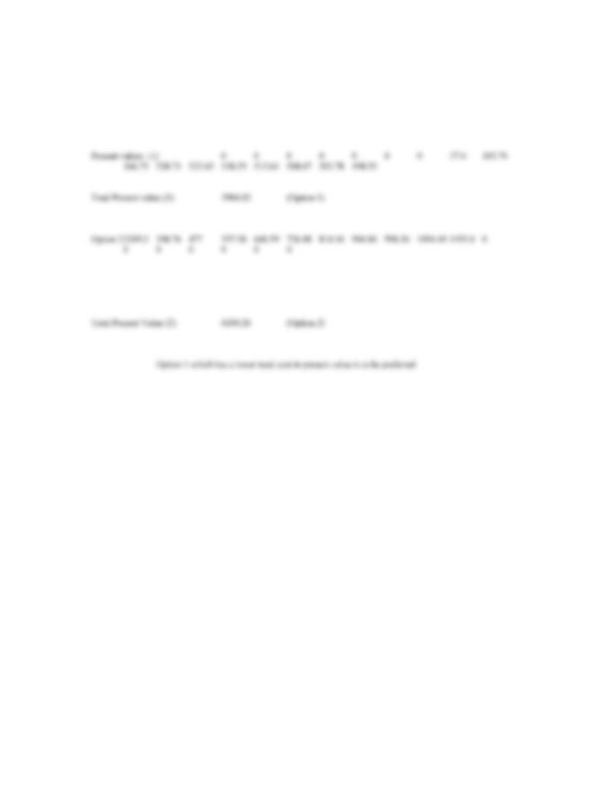
The details analysis is included in the Table 6.33 on the next page. Option #1 is to be referred.
Table 6.33 Detailed Analysis of Problems 6.12
Price escalation = 3%
Interest rate = 0.04
Life Expectancy: A = 11 B = 18
A
B
12
Discount factor 1.04 1.0816 1.124864 1.169859 1.216653 1.265319
1.315932 1.368569 1.4233118 1.480244 1.539454 1.60103
1.665074 1.7316764 1.800944 1.87298 1.9479005
Present Value (2) 383.42 441.01 495.69 547.58 596.79 643.43 687.6 729.42 768.97
806.35