Chapter 6 Homework To guarantee an absolute error of no greater than

16. R4

0x√x2+ 9dx

Consider the deﬁnite integral

The table below lists composite two-point Gaussian quadrature rule approximations

hGQ2h|e2h/eh|GQ3h|e2h/eh|

2 32.6704688953288 32.6666385097827

In Exercises 17 – 24, approximate the value of the indicated deﬁnite integral

using the composite two-point Gaussian quadrature rule and the composite

three-point Gaussian quadrature rule. For each method, use the smallest value

of nwhich will guarantee an absolute error of no greater than 5 ×10−5.

17. R2

1

xdx

Let f(x) = 1

x. Then

To guarantee an absolute error of no greater than 5×10−5from the composite

two-point Gaussian quadrature rule, the value of nmust be selected to satisfy the

Gaussian Quadrature 19

To guarantee an absolute error of no greater than 5×10−5from the composite

three-point Gaussian quadrature rule, the value of nmust be selected to satisfy the

18. R1

0e−xdx

Let f(x) = e−x. Then

To guarantee an absolute error of no greater than 5×10−5from the composite

two-point Gaussian quadrature rule, the value of nmust be selected to satisfy the

To guarantee an absolute error of no greater than 5×10−5from the composite

three-point Gaussian quadrature rule, the value of nmust be selected to satisfy the

19. R1

0tan−1xdx

Let f(x) = tan−1x. Then

20 Section 6.6

To guarantee an absolute error of no greater than 5×10−5from the composite

two-point Gaussian quadrature rule, the value of nmust be selected to satisfy the

inequality

To guarantee an absolute error of no greater than 5×10−5from the composite

three-point Gaussian quadrature rule, the value of nmust be selected to satisfy the

20. R2

1

sin x

xdx

Let f(x) = sin x

x. Then

The solution of this inequality is n≥0.90; therefore, we use n= 1. With n= 1,

the composite two-point Gaussian quadrature rule gives

Gaussian Quadrature 21

21. R1

0

1

√1+x4dx

Let f(x) = 1

√1+x4. Then

The solution of this inequality is n≥3.40; therefore, we use n= 4. With n= 4,

22. R4

0x√x2+ 9dx

Let f(x) = x√x2+ 9. Then

22 Section 6.6

The solution of this inequality is n≥6.60; therefore, we use n= 7. With n= 7,

To guarantee an absolute error of no greater than 5×10−5from the composite

three-point Gaussian quadrature rule, the value of nmust be selected to satisfy the

23. R1

0√1 + x3dx

Let f(x) = √1 + x3. Then

To guarantee an absolute error of no greater than 5×10−5from the composite

two-point Gaussian quadrature rule, the value of nmust be selected to satisfy the

To guarantee an absolute error of no greater than 5×10−5from the composite

three-point Gaussian quadrature rule, the value of nmust be selected to satisfy the

24. R1

0e−x4dx

Let f(x) = e−x4. Then

To guarantee an absolute error of no greater than 5×10−5from the composite

two-point Gaussian quadrature rule, the value of nmust be selected to satisfy the

inequality

To guarantee an absolute error of no greater than 5×10−5from the composite

three-point Gaussian quadrature rule, the value of nmust be selected to satisfy the

inequality

25. Consider the deﬁnite integral Rb

asin(√πx)dx. Numerically determine the rate

of convergence of the composite two-point Gaussian quadrature rule for each of

the following integration intervals.

(a) [a, b] = [0,1] (b) [a, b] = [π/4,9π/4] (c) [a, b] = [π, 2π]

(d) Explain any variation among the rates of convergence obtained in parts

(a), (b) and (c).

(a) Consider the deﬁnite integral

24 Section 6.6

(b) Consider the deﬁnite integral

The table below lists composite two-point Gaussian quadrature rule approxi-

mations to I(f)for several values of h. Observe that the ratio

approaches 16 as his decreased. Because 16 = 24, numerical evidence sug-

gests that the rate of convergence is O(h4).

hGQ2h

GQ2h−GQ2h/2

GQ2h/2−GQ2h/4

π−1.25496822449584 9.893

(c) Consider the deﬁnite integral

The table below lists composite two-point Gaussian quadrature rule approxi-

mations to I(f)for several values of h. Observe that the ratio

Gaussian Quadrature 25

hGQ2h

GQ2h−GQ2h/2

GQ2h/2−GQ2h/4

π/2 −1.86041349191865 15.417

26. Repeat Exercise 25 for the composite three-point Gaussian quadrature rule.

(a) Consider the deﬁnite integral

The table below lists composite three-point Gaussian quadrature rule approx-

imations to I(f)for several values of h. Observe that the ratio

approaches 2.83 as his decreased. Because log22.83 ≈1.5, numerical evi-

dence suggests that the rate of convergence is O(h1.5).

hGQ3h

GQ3h−GQ3h/2

GQ3h/2−GQ3h/4

1/2 0.851333027346831 2.864

(b) Consider the deﬁnite integral

The table below lists composite three-point Gaussian quadrature rule approx-

imations to I(f)for several values of h. Observe that the ratio

26 Section 6.6

hGQ3h

GQ3h−GQ3h/2

GQ3h/2−GQ3h/4

π−1.27232688815450 19.457

π/2−1.27319353902208 31.119

(c) Consider the deﬁnite integral

The table below lists composite three-point Gaussian quadrature rule approx-

imations to I(f)for several values of h. Observe that the ratio

approaches 64 as his decreased. Because 64 = 26, numerical evidence sug-

gests that the rate of convergence is O(h6).

hGQ3h

GQ3h−GQ3h/2

GQ3h/2−GQ3h/4

π/2 −1.86055512087582 58.004

(d) The rate of convergence is lower than expected in part (a) because the deriva-

27. Consider the deﬁnite integral Rb

ax2e−xdx. Numerically determine the rate of

convergence of the composite two-point Gaussian quadrature rule for each of

the following integration intervals.

(a) [a, b] = [0,2] (b) [a, b] = [3 −√3,3 + √3] (c) [a, b] = [−1,1]

(d) Explain any variation among the rates of convergence obtained in parts

(a), (b) and (c).

(a) Consider the deﬁnite integral

Gaussian Quadrature 27

The table below lists composite two-point Gaussian quadrature rule approx-

hGQ2h|e2h/eh|

1 0.645331215600540

(b) Consider the deﬁnite integral

The table below lists composite two-point Gaussian quadrature rule approx-

hGQ2h|e2h/eh|

√31.43104403050920

(c) Consider the deﬁnite integral

−1

The table below lists composite two-point Gaussian quadrature rule approx-

hGQ2h|e2h/eh|

1 0.871352205208655

28 Section 6.6

Optional Material

28. (a) Find the abscissas, xi, and the weights, wi, of the three-point Gauss-

Hermite quadrature formula

Z∞

−∞

e−x2f(x)dx ≈w1f(x1) + w2f(x2) + w3f(x3).

Use the fact that the Hermite polynomials, Hn(x), are orthogonal in the

corresponding inner product

(f, g) = Z∞

−∞

e−x2f(x)g(x)dx

and that H3(x) = 8x3−12x. Find the weights by undetermined coefficients

using the values:

Z∞

−∞

e−x2dx =√πZ∞

−∞

xe−x2dx = 0 Z∞

−∞

x2e−x2dx =√π

2.

(b) Use your results from part (a) to evaluate both

Z∞

−∞

e−x2

1 + x2dx and Z∞

−∞

1

1 + x2dx.

(a) The abscissas for the three-point Gauss-Hermite quadrature rule are the roots

To determine the weights, we note that the three-point Gauss-Hermite quadra-

ture rule has degree of precision equal to ﬁve; thus, the quadrature rule must

w1+w2+w3=√π

Gaussian Quadrature 29

whose solution is

w1=√π

6, w2=2√π

3,and w3=√π

6.

Thus,

Z∞

−∞

e−x2f(x)dx ≈√π

6f −r3

2!+2√π

3f(0) + √π

6f r3

2!.

(b) For

Z∞

−∞

e−x2

1 + x2dx,

f(x) = 1

1+x2. Thus,

29. (a) Find the abscissas, xi, and the weights, wi, of the three-point Gauss-

Chebyshev quadrature formula

Z1

−1

f(x)

√1−x2dx ≈w1f(x1) + w2f(x2) + w3f(x3).

Use the fact that the Chebyshev polynomials, Tn(x), are orthogonal in the

corresponding inner product

(f, g) = Z1

−1

f(x)g(x)

√1−x2dx

and that T3(x) = 4x3−3x. Find the weights by undetermined coefficients

using the values:

Z1

−1

1

√1−x2dx =πZ1

−1

x

√1−x2dx = 0 Z1

−1

x2

√1−x2dx =π

2.

30 Section 6.6

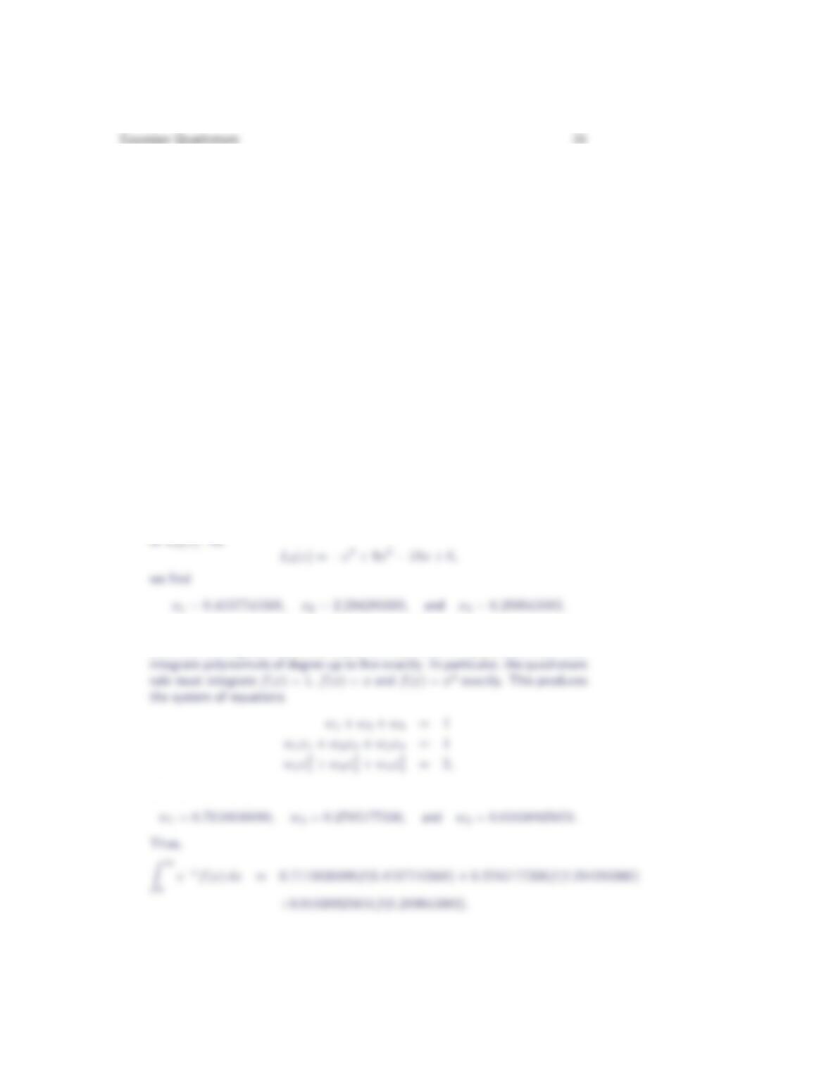
(b) Use your results from part (a) to evaluate

Z1

−1

cos x

√1−x2dx.

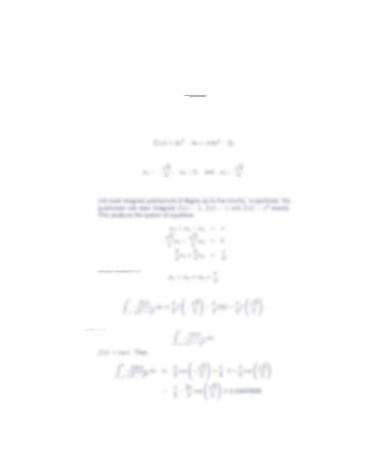
(a) The abscissas for the three-point Gauss-Chebyshev quadrature rule are the

roots of T3(x). As

it follows that

2, x2= 0,and x3=√3

2.

To determine the weights, we note that the three-point Gauss-Chebyshev

quadrature rule has degree of precision equal to ﬁve; thus, the quadrature

Thus,

(b) For

30. (a) Find the abscissas, xi, and the weights, wi, of the three-point Gauss-

Laguerre quadrature formula

Z∞

0

e−xf(x)dx ≈w1f(x1) + w2f(x2) + w3f(x3).

Use the fact that the Laguerre polynomials, Ln(x), are orthogonal in the

corresponding inner product

(f, g) = Z∞

0

e−xf(x)g(x)dx

and that L3(x) = −x3+ 9x2−18x+ 6. Find the weights by undetermined

coefficients using the values:

Z∞

0

e−x= 1 Z∞

0

xe−x= 1 Z∞

0

x2e−x= 2.

(b) Use your results from part (a) to evaluate both

Z∞

0

e−x

1 + x2dx and Z∞

0

1

1 + x2dx.

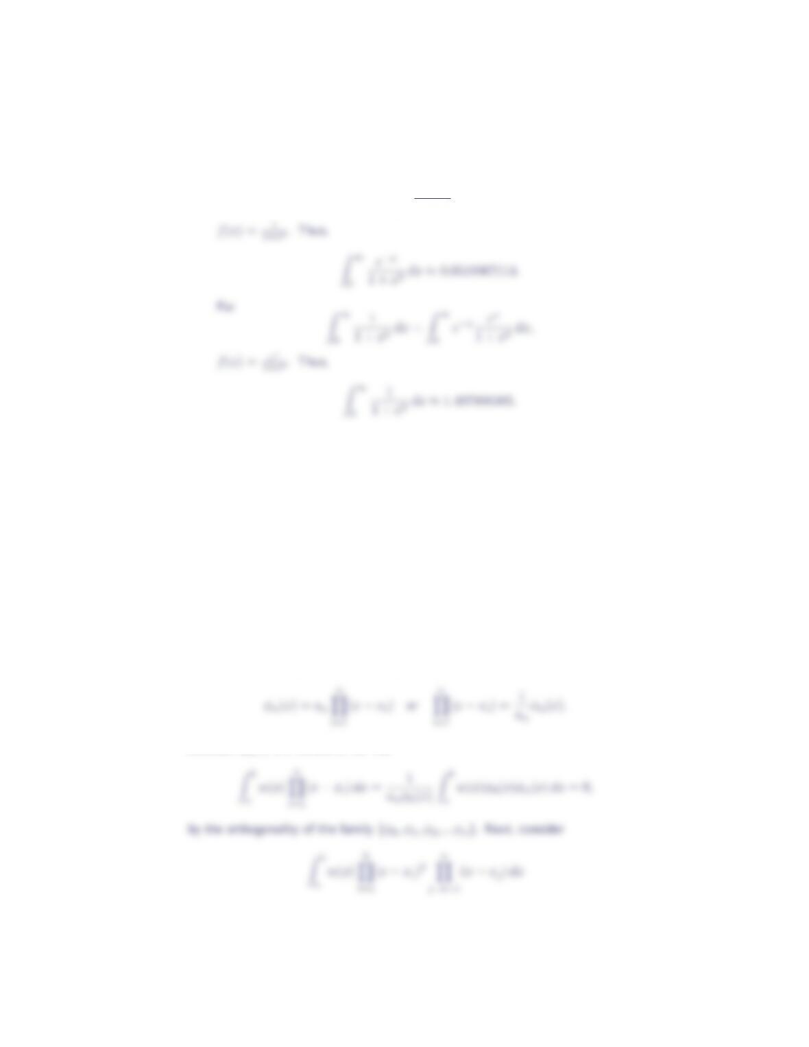
(a) The abscissas for the three-point Gauss-Laguerre quadrature rule are the roots

To determine the weights, we note that the three-point Gauss-Laguerre quadra-

ture rule has degree of precision equal to ﬁve; thus, the quadrature rule must

whose solution is

32 Section 6.6

(b) For

Z∞

0

e−x

1 + x2dx,

31. Let wbe a weight function on [a, b], let {φ0, φ1, φ2, …φn} ⊂ Πnbe an orthogonal

family with respect to wwith degree of φk=kfor each kand let x1,x2,x3, …,

xnbe the roots of φn(x). Show that

Zb

a

w(x)

n

Y

i=1

(x−xi)dx = 0

and

Zb

a

w(x)

k

Y

i=1

(x−xi)2

n

Y

j=k+1

(x−xj)dx = 0

for k= 1,2,3, …, n −1.

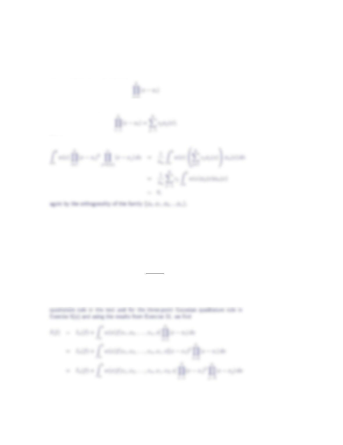
Suppose the leading coefficient of φn(x)is an. Then

Because φ0(x)is a constant, we ﬁnd

Gaussian Quadrature 33

for k= 1,2,3, …, n −1. Because

is a polynomial of degree k < n, there exist constants c1,c2,c3, …, cksuch that

Thus,

32. Let wbe a weight function on [a, b], let nbe a positive integer, let {φ0, φ1, φ2, …, φn} ⊂

Πnbe an orthogonal family with respect to wwith degree of φk=kfor each k

and let In(f) denote the corresponding Gaussian quadrature rule for approxi-

mating

I(f) = Zb

a

f(x)w(x)dx.

Suppose fhas 2ncontinuous derivatives. Show there exists ξ∈[a, b] such that

I(f) = In(f) + αn

a2

n(2n)!f(2n)(ξ),

where αn=Rb

aφ2

n(x)w(x)dx and anis the leading coefficient of φn(x).

Following the procedure used to derive the error term for the two-point Gaussian

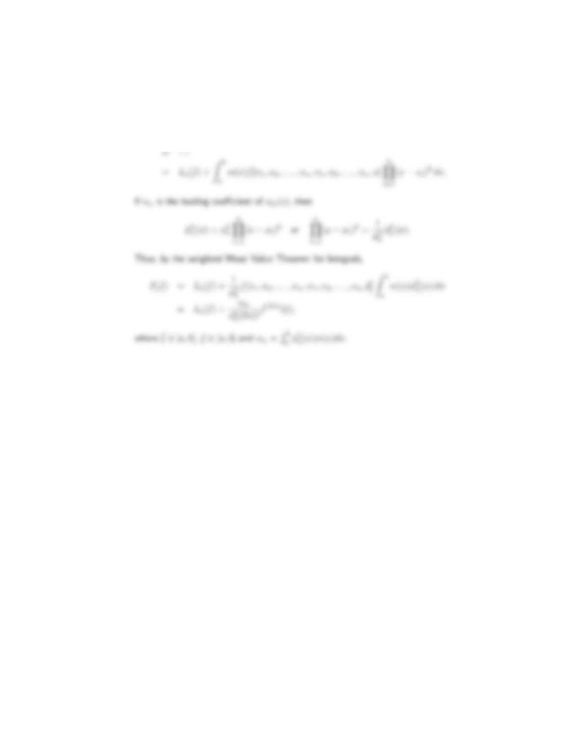
34 Section 6.6

=In(f) + Zb

a

w(x)f[x1, x2, . . . , xn, x1, x2, x3, x]

3

Y

i=1

(x−xi)2

n

Y

j=4

(x−xj)dx