Chapter 6 Homework The Solution This Inequality 417454 Therefore

12 Section 6.8

using 81 function evaluations. To guarantee an absolute error of no greater than

11. R2

0e−xsin(x2cos e−x)dx

Using the adaptive Simpson’s rule with ǫ= 5 ×10−7, we find

Thus, to guarantee an absolute error of no greater than 5×10−7from the composite

Simpson’s rule, the value of nmust be selected to satisfy the inequality

Using the adaptive Simpson’s rule with ǫ= 5 ×10−11, we find

12. R1

0√1 + x4dx

Adaptive Quadrature 13

Using the adaptive Simpson’s rule with ǫ= 5 ×10−7, we find

Thus, to guarantee an absolute error of no greater than 5×10−7from the composite

Simpson’s rule, the value of nmust be selected to satisfy the inequality

Using the adaptive Simpson’s rule with ǫ= 5 ×10−11, we find

13. R1

0

u7

1+u14 du

Using the adaptive Simpson’s rule with ǫ= 5 ×10−7, we find

The solution of this inequality is n≥91.25; therefore, we use n= 92, and 93

function evaluations are needed from the composite Simpson’s rule.

Using the adaptive Simpson’s rule with ǫ= 5 ×10−11, we find

Z1

0

u7

1 + u14 du ≈0.09597143321

using 537 function evaluations. To guarantee an absolute error of no greater than

5×10−11 from the composite Simpson’s rule, the value of nmust be selected to

satisfy the inequality

(1 −0)5

180n4·6240.27 ≤5×10−11.

The solution of this inequality is n≥912.52; therefore, we use n= 914 (remember

that Simpson’s rule requires an even number of subintervals), and 915 function

evaluations are needed from the composite Simpson’s rule.

14. R10

025e−25xdx

Using the adaptive Simpson’s rule with ǫ= 5 ×10−7, we find

Thus, to guarantee an absolute error of no greater than 5×10−7from the composite

Simpson’s rule, the value of nmust be selected to satisfy the inequality

Adaptive Quadrature 15

15. R1

0

1

1+exdx

Using the adaptive Simpson’s rule with ǫ= 5 ×10−7, we find

Thus, to guarantee an absolute error of no greater than 5×10−7from the composite

Simpson’s rule, the value of nmust be selected to satisfy the inequality

Using the adaptive Simpson’s rule with ǫ= 5 ×10−11, we find

16. Rπ

0cos(cos x+ 3 sin x+ 2 cos(2x) + 3 cos(3x) + 3 sin(2x))dx

Using the adaptive Simpson’s rule with ǫ= 5 ×10−7, we find

Zπ

16 Section 6.8

Thus, to guarantee an absolute error of no greater than 5×10−7from the composite

Simpson’s rule, the value of nmust be selected to satisfy the inequality

17. (a) Evaluate the integral

Z1

0

sin(√πx)dx

to six decimal places of accuracy using the adaptive Simpson’s rule. How

many function evaluations were needed?

(b) Make the change of variable u2=πx in the integral from part (a) and

re-evaluate using the adaptive Simpson’s rule. How does the number of

function evaluations compare with the number from part (a)?

(a) With ǫ= 5 ×10−7, we find

(b) With the change of variable u2=πx,

Adaptive Quadrature 17

using 33 function evaluations. By eliminating the discontinuities in the deriva-

tives of the integrand, we achieved nearly a five-fold reduction in the number

of function evaluations.

18. (a) Evaluate the integral

Z1

0

2

2 + sin(10πx)dx

to ten decimal places of accuracy using the adaptive Simpson’s rule. How

many function evaluations were needed?

(b) Recognizing that the integrand in part (a) is periodic with period 1/5,

recompute the value from part (a) as

5Z0.2

0

2

2 + sin(10πx)dx

using the adaptive Simpson’s rule. How does the number of function eval–

uations compare with the number from part (a)?

(a) With ǫ= 5 ×10−11, we find

(b) Recognizing that the integrand in part (a) is periodic with period 1/5, we

rewrite the integral as

19. The Fresnel integrals

c(x) = Zx

0

cos π

2t2dt s(x) = Zx

0

sin π

2t2dt

18 Section 6.8

(a) Construct a table of values for c(x) and s(x) for xranging from 0 through

2 in increments of 0.2. Each entry in the table should be accurate to five

decimal places.

(b) Determine the two smallest positive values for xsuch that c(x) = 0.5,

accurate to four decimal places. Repeat for the equation s(x) = 0.5.

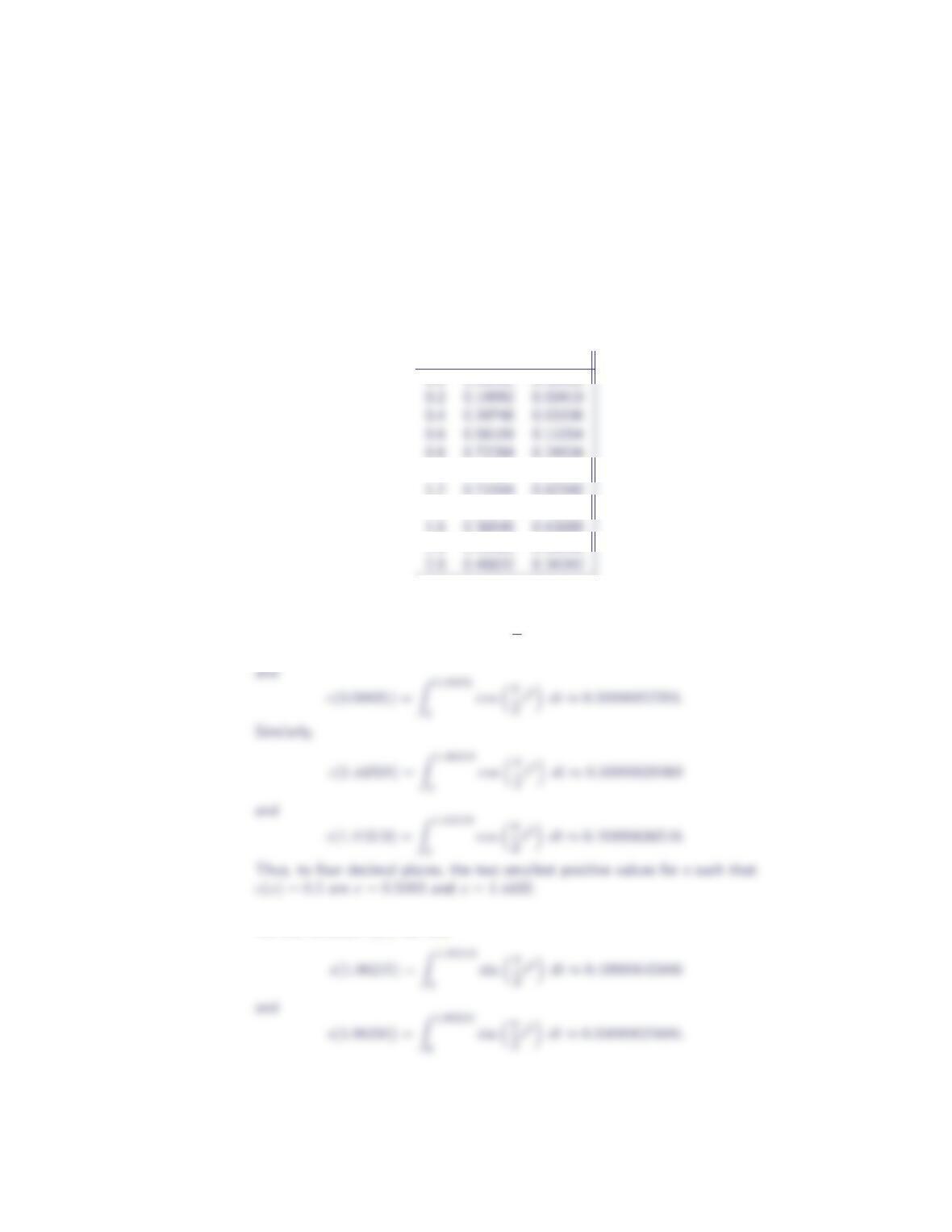
(a) Using the adaptive Simpson’s rule with ǫ= 5 ×10−6, we generate the table

xc(x)s(x)

0.0 0.00000 0.00000

1.0 0.77989 0.43826

1.4 0.54310 0.71352

1.8 0.33363 0.45094

(b) Using the adaptive Simpson’s rule with ǫ= 5 ×10−11, we find

c(0.50830) = Z0.50830

0

cos π

2t2dt ≈0.49999138625

For the function s(x), we find

Adaptive Quadrature 19

Similarly,

s(1.74938) = Z1.74938

0

sin π

2t2dt ≈0.50000179149

and

s(1.74939) = Z1.74939

0

sin π

2t2dt ≈0.49999183638.

Thus, to four decimal places, the two smallest positive values for xsuch that

s(x) = 0.5are x= 1.0622 and x= 1.7494.

20. Consider the integral

Zx

0

sin t

tdt.

(a) Use the adaptive two-point Gaussian quadrature scheme to tabulate the

value of this integral for xranging from 0 through 10 in increments of 0.5.

Each tabulated value should be accurate to six decimal places.

(b) What happens if you try to use the adaptive Simpson’s rule to tabulate the

values of this integral? Can you think of a way to alleviate this problem?

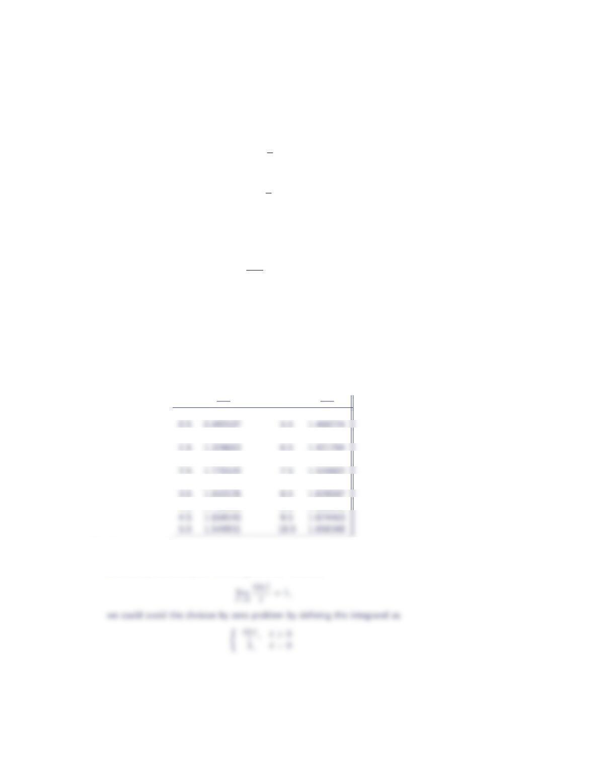
(a) Using the adaptive two-point Gaussian quadrature rule with ǫ= 5 ×10−7, we

generate the table

xRx

0

sin t

tdt xRx

0

sin t

tdt

0.0 0.000000

1.0 0.946083 6.0 1.424688

2.0 1.605413 7.0 1.454597

3.0 1.848652 8.0 1.574187

4.0 1.758203 9.0 1.665040

(b) The adaptive Simpson’s rule will attempt to evaluate the integrand at t= 0.

Unfortunately, the integrand is not defined at t= 0 due to division by zero, so

a divide by zero exception will be generated. Because

21. Evaluate

R1/2

0e2(1−x)3/3dx

R1

0e2(1−x)3/3dx and R1/2

0e−x2+2x3/3dx

R1

0e−x2+2x3/3dx .

These expressions arise in determining the probability that an allele with a

selective advantage over its competitors will become fixed in a population (see

P.D. Taylor and A. Sauer, “The Selective Advantage of Sex-Ratio Homeostasis,”

American Naturalist, 116, 305 – 310, 1980).

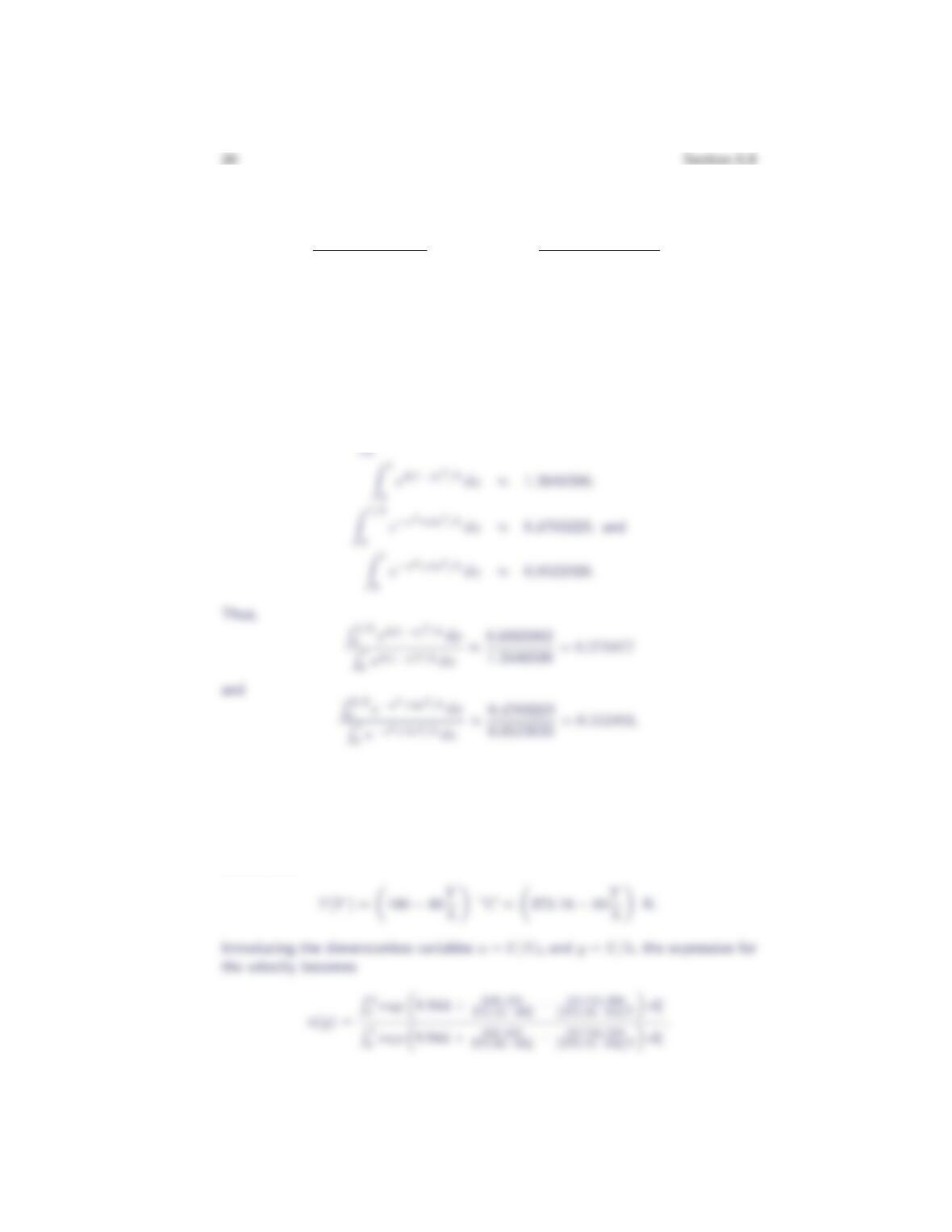
Using the adaptive Simpson’s rule with ǫ= 5 ×10−7, we find

Z1/2

e2(1−x)3/3dx ≈0.6933902;

22. Rework the “Flow Between Parallel Plates” problem assuming that the lower

plate is maintained at 100◦Cand the upper plate is maintained at 20◦C.

With the assumption of a linear temperature gradient between the two plates, it

follows that

Adaptive Quadrature 21

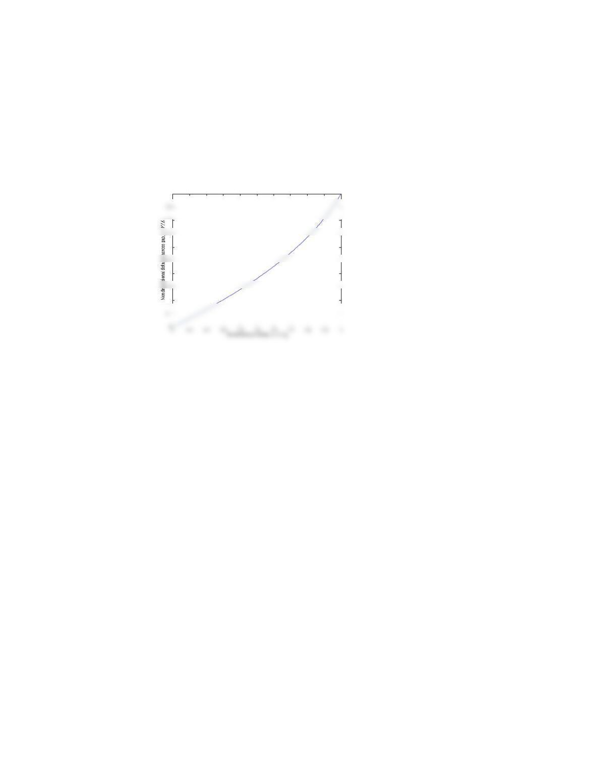
The figure below displays the nondimensional velocity distribution. To produce this

graph, values of uwere calculated at yi= 0.01ifor i= 0,1,2, …, 100. All integrals

were evaluated using adaptive three-point Gaussian quadrature with ǫ= 5 ×10−7.

The independent variable has been plotted along the vertical axis to match the

geometry depicted in Figure 6.14(a).

0.2

0.4

0.6

0.8

1