Romberg Integration 1
6.7 Romberg Integration
1. Romberg integration approximates the value of the integral
Z1
0
1
1 + x2dx
with an error of 1.2113 ×10⁻¹¹ using only 33 function evaluations. How many
function evaluations would be needed to achieve the same level of accuracy using
the composite trapezoidal rule, the composite midpoint rule, the composite
Simpson’s rule and the composite two-point Gaussian quadrature rule?
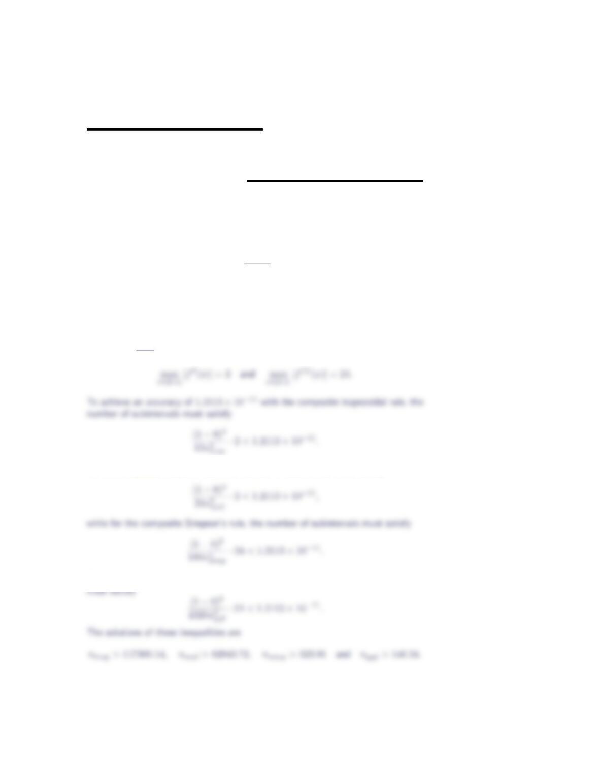
Let f(x) = 1
1+x2. Then
For the composite midpoint rule, the number of subintervals must satisfy
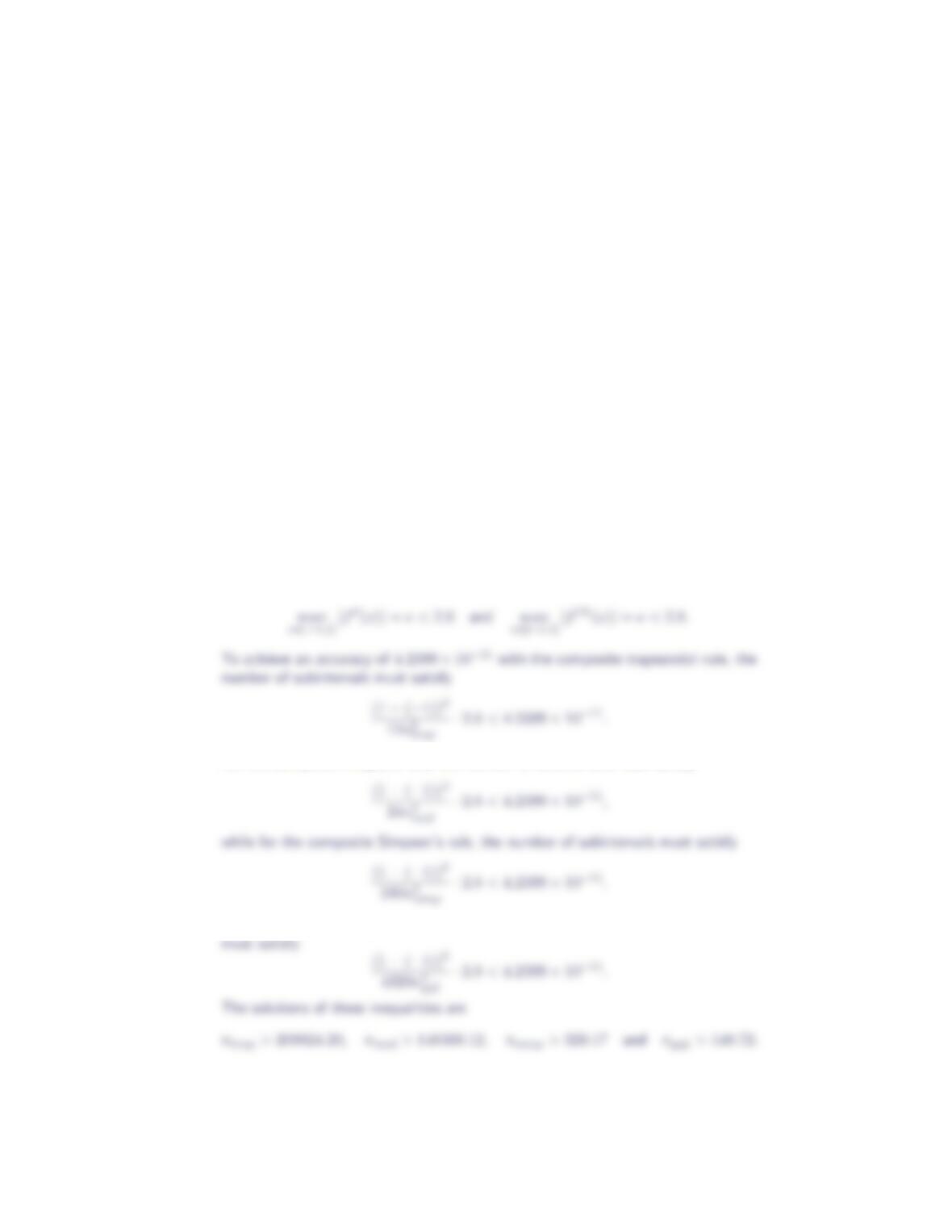
For the composite two-point Gaussian quadrature rule, the number of subintervals
2Section 6.7
Recall that the number of function evaluations used by the composite trapezoidal
rule and the composite Simpson’s rule is one more than the number of subintervals,
the number of function evaluations used by the composite midpoint rule is equal
to the number of subintervals, and the number of function evaluations used by the
composite two-point Gaussian quadrature rule is twice the number of subintervals.
Thus, to achieve an accuracy of 1.2113 ×10⁻¹¹, the composite trapezoidal rule
would need 117302 function evaluations, the composite midpoint rule would need
82944 function evaluations, the composite Simpson’s rule would need 325 function
evaluations and the composite two-point Gaussian quadrature rule would need 294
function evaluations.
2. Romberg integration approximates the value of the integral
Z1
−1
e−xdx
with an error of 4.2399 ×10⁻¹¹ using only 17 function evaluations. How many
function evaluations would be needed to achieve the same level of accuracy using
the composite trapezoidal rule, the composite midpoint rule, the composite
Simpson’s rule and the composite two-point Gaussian quadrature rule?
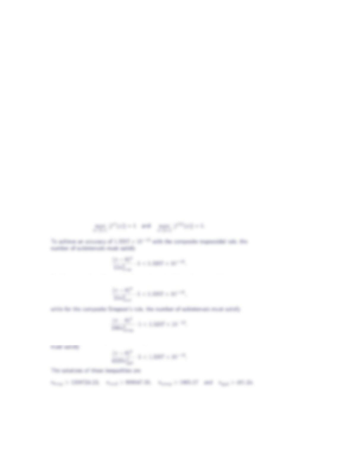
Let f(x) = e−x. Then
For the composite midpoint rule, the number of subintervals must satisfy
For the composite two-point Gaussian quadrature rule, the number of subintervals
Romberg Integration 3
Recall that the number of function evaluations used by the composite trapezoidal
rule and the composite Simpson’s rule is one more than the number of subintervals,
the number of function evaluations used by the composite midpoint rule is equal
to the number of subintervals, and the number of function evaluations used by the
composite two-point Gaussian quadrature rule is twice the number of subintervals.
Thus, to achieve an accuracy of 4.2399 ×10⁻¹¹, the composite trapezoidal rule
would need 209826 function evaluations, the composite midpoint rule would need
148369 function evaluations, the composite Simpson’s rule would need 331 function
evaluations and the composite two-point Gaussian quadrature rule would need 298
function evaluations.
3. Romberg integration approximates the value of the integral
Zπ
0
sin xdx
with an error of 1.3207 ×10⁻¹² using only 33 function evaluations. How many
function evaluations would be needed to achieve the same level of accuracy using
the composite trapezoidal rule, the composite midpoint rule, the composite
Simpson’s rule and the composite two-point Gaussian quadrature rule?
Let f(x) = sin x. Then
For the composite midpoint rule, the number of subintervals must satisfy
For the composite two-point Gaussian quadrature rule, the number of subintervals
4Section 6.7
Recall that the number of function evaluations used by the composite trapezoidal
In Exercises 4 – 7, the first column of the Romberg integration table for the
specified definite integral is provided. Complete the table and determine the
absolute error in the final approximation.
4. R3π/2
0cos xdx
2.3561944902
−0.4879838567
−0.8815735630
−0.9709165361
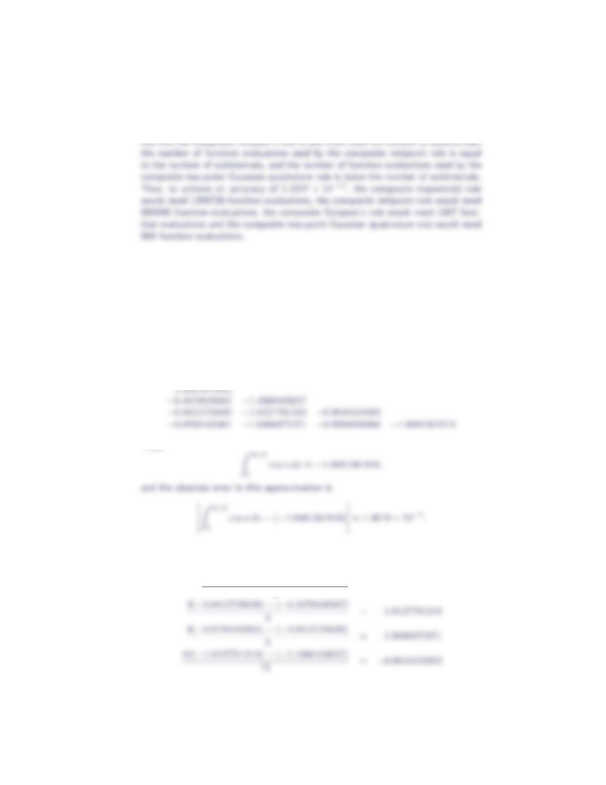
The four row Romberg integration table is
Thus,
The values in the second, third and fourth columns of the table were calculated as
4(−0.4879838567) −2.3561944902
3=−1.4360433057
Romberg Integration 5
5. R2
0exdx
8.3890560989
6.9128098779
6.5216101095
6.4222978214
The four row Romberg integration table is
Thus,
The values in the second, third and fourth columns of the table were calculated as
4(6.9128098779) −8.3890560989
16(6.3912101867) −6.4207278042
6. R4
0x√x2+ 9dx
40.0000000000
34.4222051019
33.1013022725
32.7750803748
6Section 6.7
The four row Romberg integration table is
Thus,
and the absolute error in this approximation is
The values in the second, third and fourth columns of the table were calculated as
4(34.4222051019) −40.0000000000
7. R3
1
1
xdx
1.3333333333
1.1666666667
1.1166666667
1.1032106782
The four row Romberg integration table is
1.3333333333
Romberg Integration 7
and the absolute error in this approximation is
The values in the second, third and fourth columns of the table were calculated as
4(1.1666666667) −1.3333333333
In Exercises 8 – 13:
(a) Starting with only one subinterval, construct the four row Romberg integra-
tion table for the indicated integral.
(b) What is the error estimate for the final approximation? How does this com-
pare with the actual error?
(c) How many subintervals would have been necessary to achieve the same ac-
curacy using the composite trapezoidal rule without extrapolation?
8. R3.5
3
x
√x2−4dx
(a) The four row Romberg integration table is
8Section 6.7
which compares favorably with the actual error
(c) Let f(x) = x
√x2−4. Then
9. R1
0x2e−xdx
(a) The four row Romberg integration table is
0.18393972058572
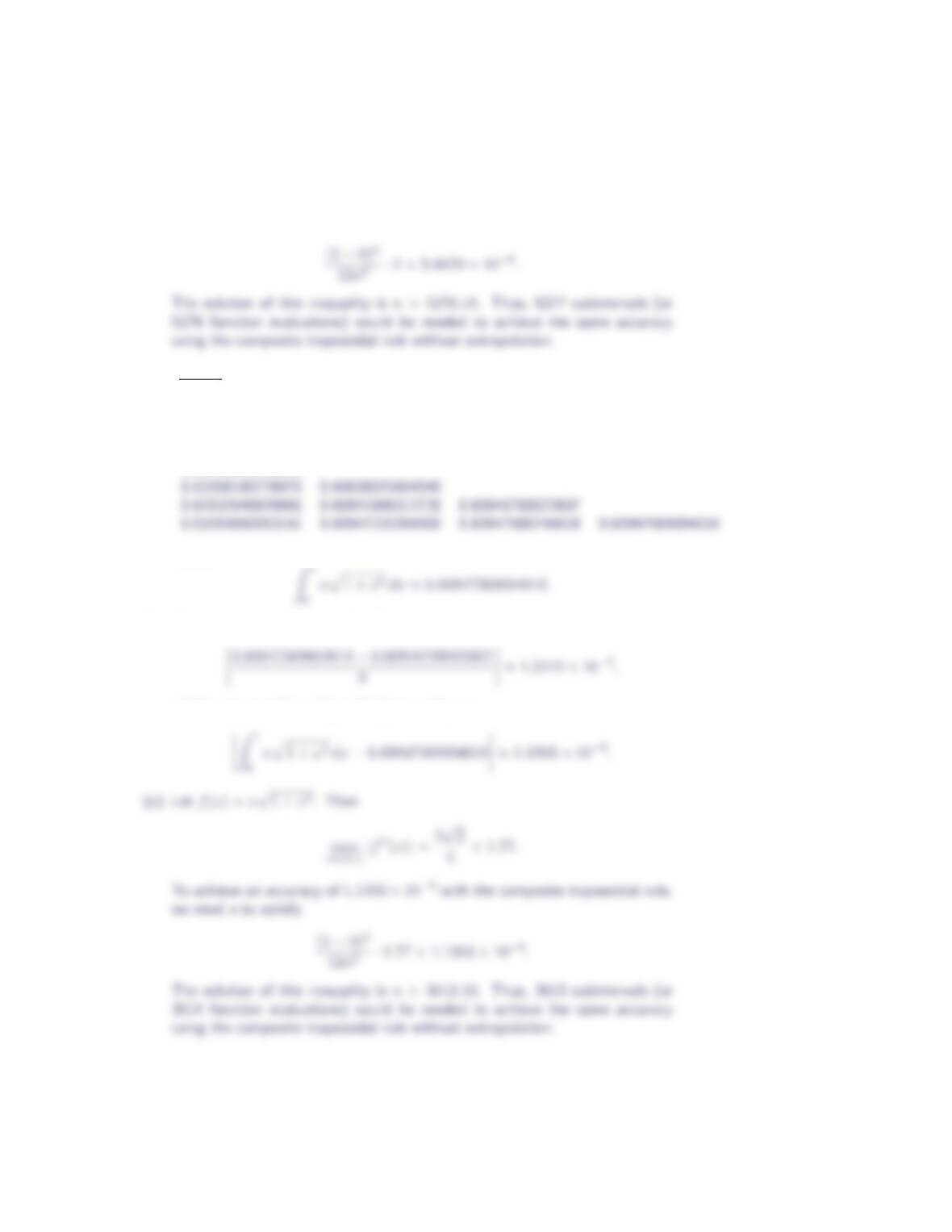
(b) The error estimate for the final Romberg integration approximation is
Romberg Integration 9
To achieve an accuracy of 5.9870 ×10⁻⁹with the composite trapezoidal rule,
we need nto satisfy
10. R1
0x√1 + x2dx
(a) The four row Romberg integration table is
0.70710678118655
Thus,
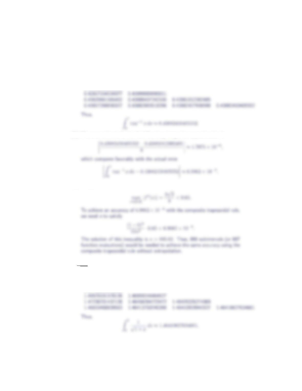
(b) The error estimate for the final Romberg integration approximation is
which compares favorably with the actual error
10 Section 6.7
11. R1
0tan−1xdx
(a) The four row Romberg integration table is
0.39269908169872
(b) The error estimate for the final Romberg integration approximation is
(c) Let f(x) = tan−1x. Then
12. R2
0
1
√1+xdx
(a) The four row Romberg integration table is
1.57735026918963
Romberg Integration 11
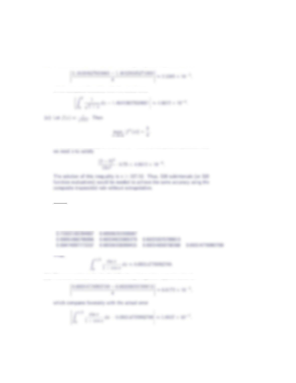
(b) The error estimate for the final Romberg integration approximation is
which compares favorably with the actual error
To achieve an accuracy of 4.6612 ×10⁻⁶with the composite trapezoidal rule,
13. Rπ/2
0
sin x
1+cos xdx
(a) The four row Romberg integration table is
0.78539816339745
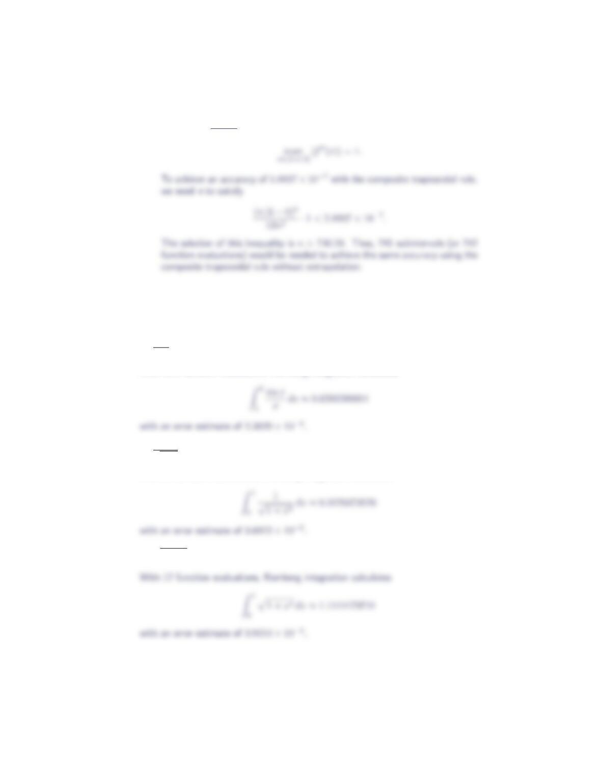
(b) The error estimate for the final Romberg integration approximation is
12 Section 6.7
(c) Let f(x) = sin x
1+cos x. Then
In Exercises 14 – 19, approximate the value of the indicated definite integral to
within an absolute error tolerance of 5 ×10⁻⁷using Romberg integration. How
many function evaluations are needed?
14. R2
1
sin x
xdx
With nine function evaluations, Romberg integration calculates
15. R1
0
1
√1+x4dx
With 17 function evaluations, Romberg integration calculates
16. R1
0√1 + x3dx
17. R1
0sin(x2)dx
Romberg Integration 13
With 17 function evaluations, Romberg integration calculates
18. R1
0
1
1+x6dx
19. R1
0x2tan−1(x4)dx
20. Use the table generated in the “Tabulating the Error Function” application
problem and Hermite cubic interpolation to approximate the value of the error
function at the indicated value of x. How well does the value obtained in this
manner compare to the actual value of the error function?
(a) x= 0.799 (b) x= 1.265 (c) x= 0.156
(d) x= 1.771 (e) x= 0.301 (f) x= 1.545
(a) Using Hermite cubic interpolation with the data corresponding to x= 0.7and
14 Section 6.7
(e) Using Hermite cubic interpolation with the data corresponding to x= 0.3and
(f) Using Hermite cubic interpolation with the data corresponding to x= 1.5and
21. Show that, for any k,Rk,2is the composite Simpson’s rule with h= (b−a)/2k−1.
Note that if Rk,1is calculated with a step size of h= (b−a)/2k−1, then Rk−1,1
is calculated with a step size of
Now, write
Romberg Integration 15
Thus,
Rk,2=h
3
f(a)+4
2k−2
X
j=1
f(a+ (2j−1)h)+2
2k−2−1
X
j=1
f(a+ 2jh) + f(b)
,
which we recognize as the composite Simpson’s rule with h= (b−a)/2k−1.
22. The table below gives the volume v(measured in cubic inches) and the pressure
p(measured in pounds per square inch) of a gas as it expands.
v0.75 1.00 1.25 1.50 1.75 2.00 2.25 2.50 2.75
p89.8 68.7 55.0 45.8 39.3 34.4 30.5 27.5 26.0
Estimate the work done by the gas,
W=Z2.75
0.75
pdv,
as follows: use the trapezoidal rule with h= 2.0, h= 1.0, h= 0.5 and h= 0.25,
and then extrapolate.
We start by computing the trapezoidal rule approximations. With h= 2.0,h= 1.0,
h= 0.5and h= 0.25, we find
respectively. The four row Romberg integration table then becomes
115.8
23. Consider the integral
ZM
exp(−ICt)
dy
y[A(1 −y)−Bln y],
16 Section 6.7
which arises in the projection printing of a photoresist film. Here, Mdenotes
the normalized photoactive compound concentration present in the resist film
after exposure to light, A,Band Care material properties of the resist film,
and the product It is the exposure energy of the light source used during the
printing phase. For the resist material AZ2400, A= 0.162/µm, B= 0.184/µm
and C= 0.0128 cm2/mJ. Suppose the exposure energy is 110 mJ/cm2.
(a) For the resist material AZ2400, evaluate the above integral for M= 0.32
to five decimal places.
(b) Determine the value of M, correct to four decimal places, so that
ZM
exp(−ICt)
dy
y[A(1 −y)−Bln y]= 1.
(a) Using Romberg integration with a tolerance of 5×10⁻⁶, we find
and