94
CHAPTER 6
REGRESSION ANALYSIS
ANSWERS TO PROBLEMS AND CASES
2. a. If GNP is increased by 1 billion dollars, we will expect earnings to increase
The regression equation is
Analysis of Variance
Source DF SS MS F P
a. Yes, the regression is significant. Reject
0:
H
using either the t value 2.384
4. Correlation of Time and Value = 0.967
The regression equation is
Predictor Coef SE Coef T P
Analysis of Variance
Source DF SS MS F P
.
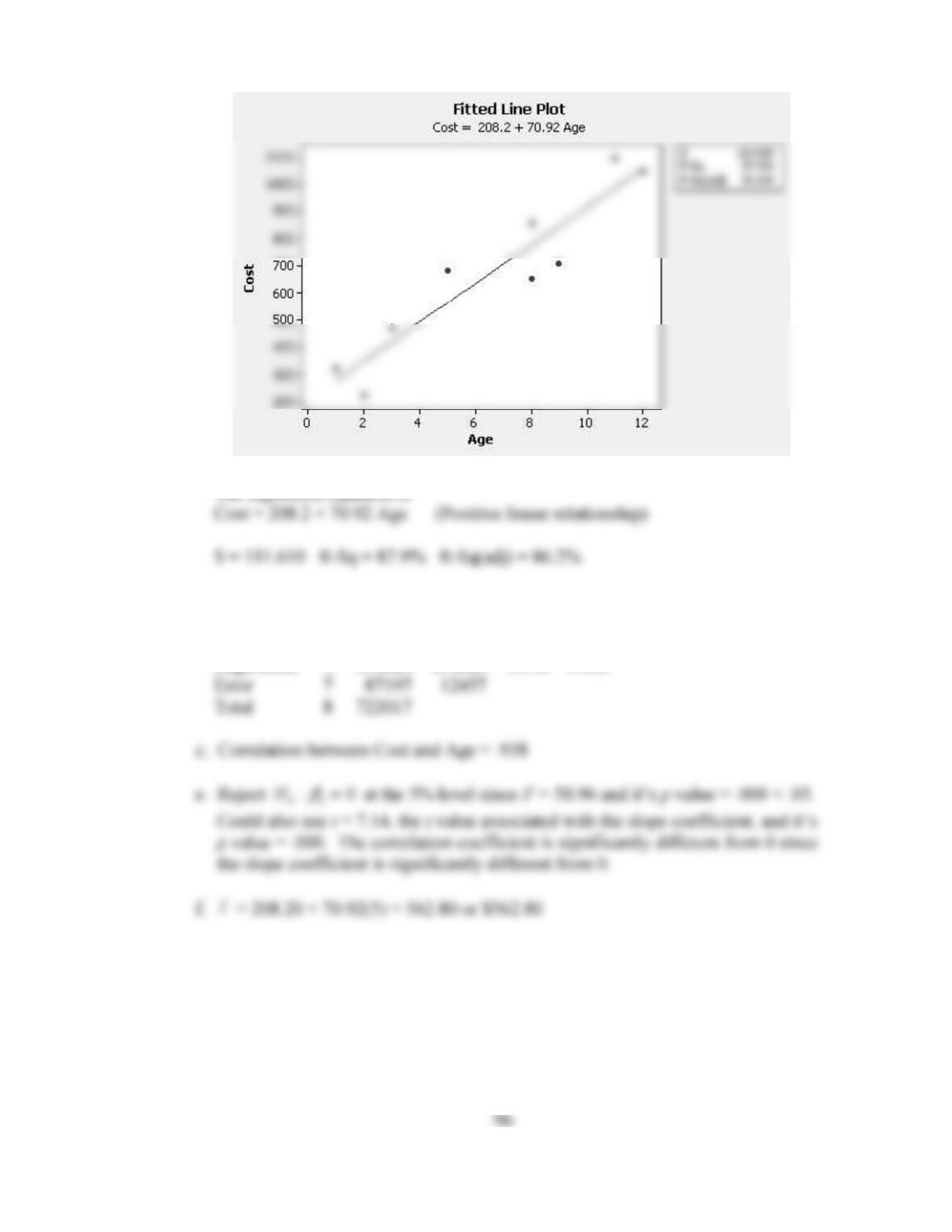
Analysis of Variance
Source DF SS MS F P
Regression 1 634820 634820 50.96 0.000
6. a, b and d.
97
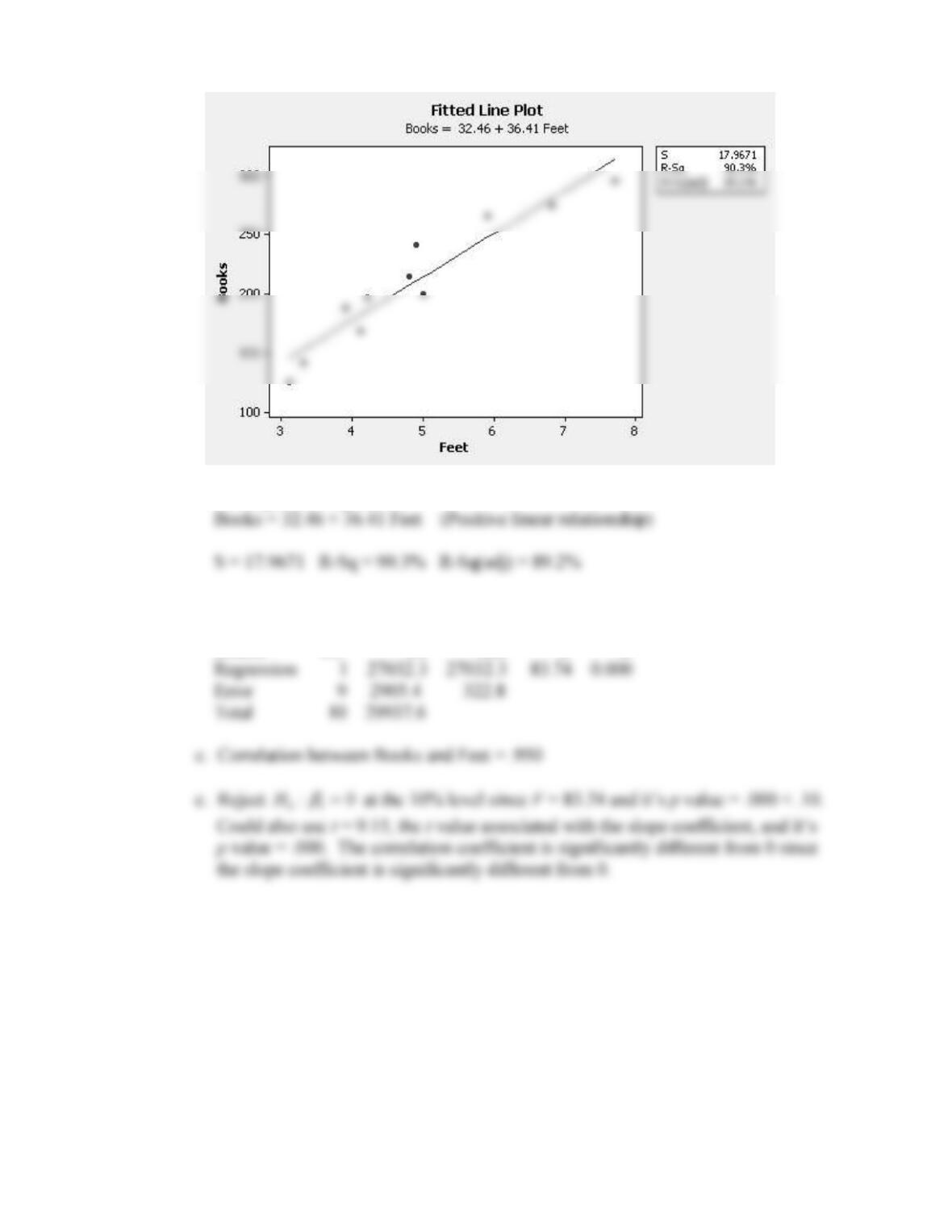
The regression equation is
Analysis of Variance
Source DF SS MS F P
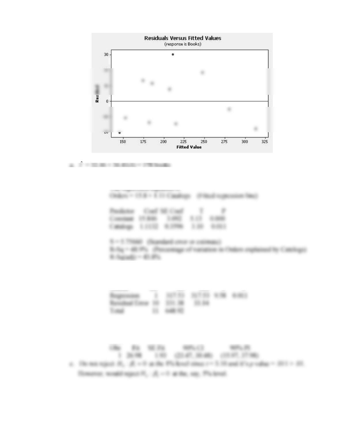
f. Based on the residuals versus the fitted values plot, there is no reason to
doubt the adequacy of the simple linear regression model.
98
g.
7. a, b, c & d.
Analysis of Variance (ANOVA Table)
Source DF SS MS F P
Predicted Values for New Observations
New
99
Predictor Coef SE Coef T P
Analysis of Variance
Source DF SS MS F P
b. The data set is small. Moreover, r2 = .49 so only 49% of the variation in investment
100
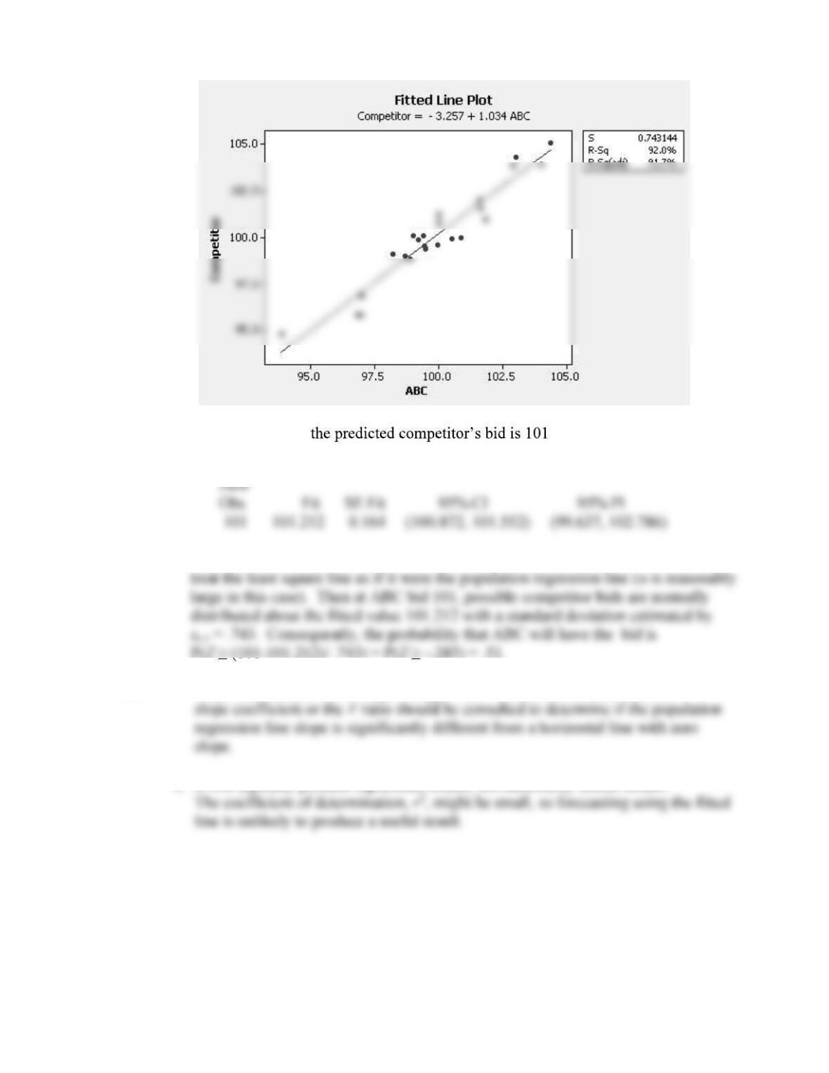
b. If ABC bids 1.01, .212. A 95% prediction
interval (PI) is given below.
c. Assume normality distributed errors about the population regression line and
10. a. Only if the sample size is large enough. The t statistic associated with the
b. It will typically produce significant results, not necessarily useful results.
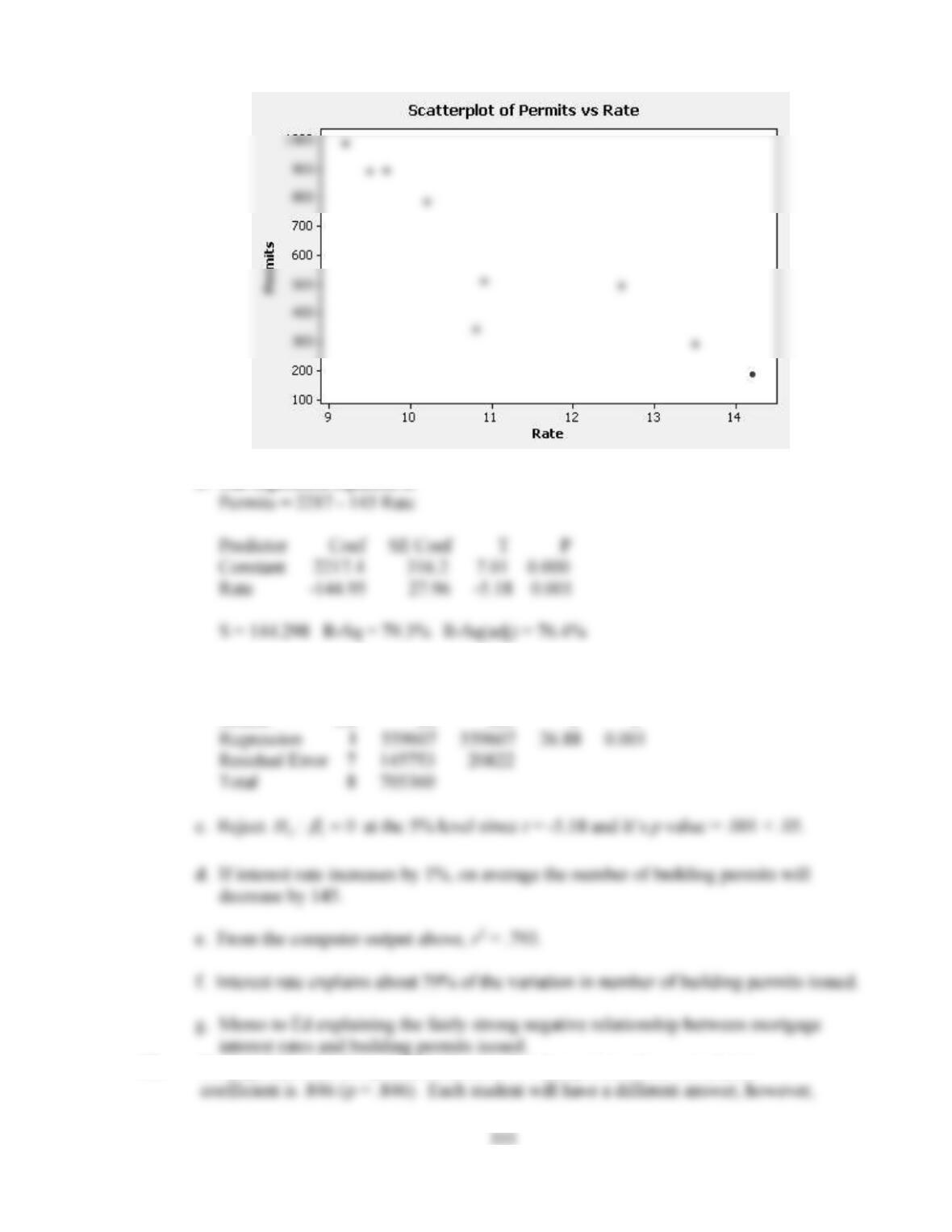
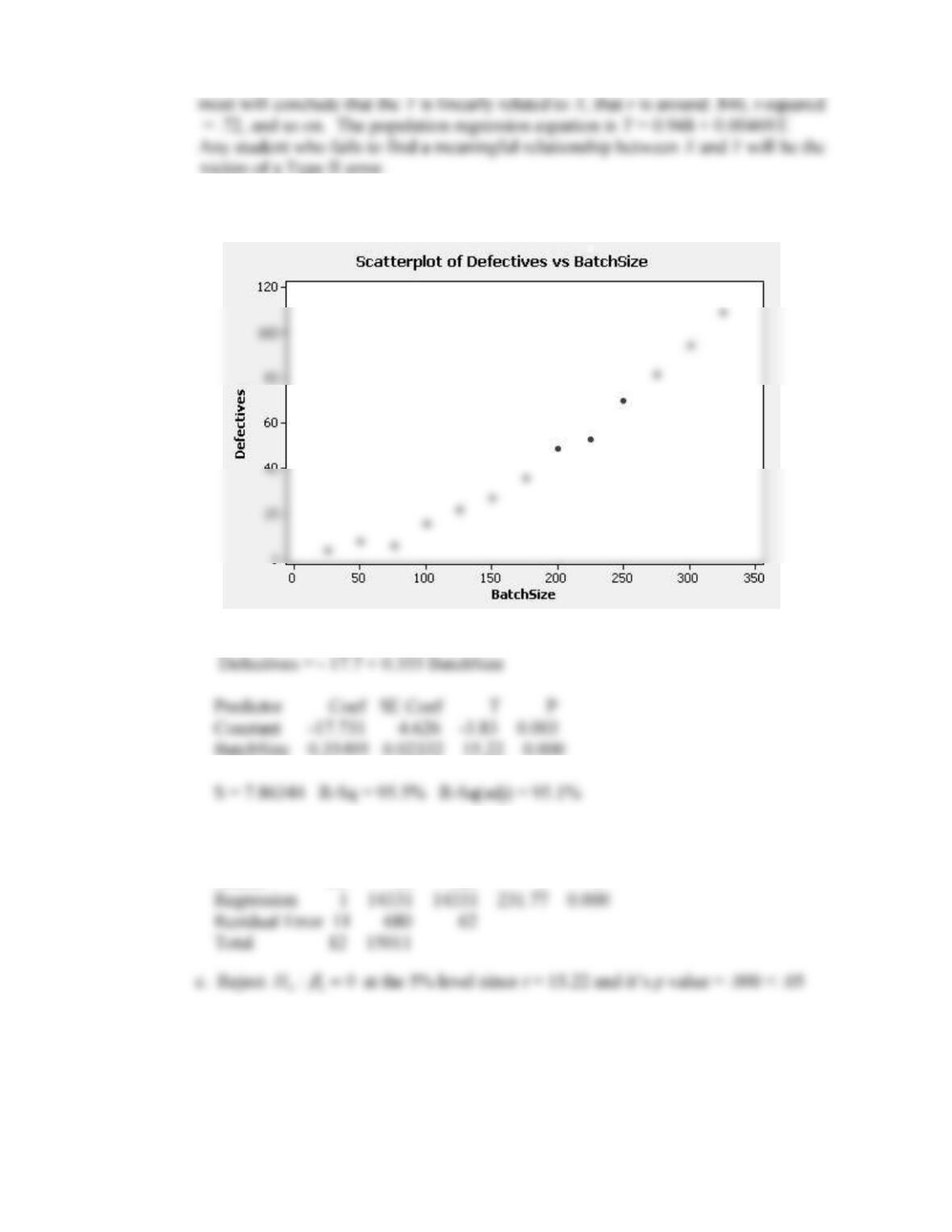
11. a. Scatter diagram follows.
b. The regression equation is
Analysis of Variance
Source DF SS MS F P
12. The population for this problem contains X–Y data points whose correlation
102
13. a. Scatter diagram follows.
b. The regression equation is
Analysis of Variance
Source DF SS MS F P
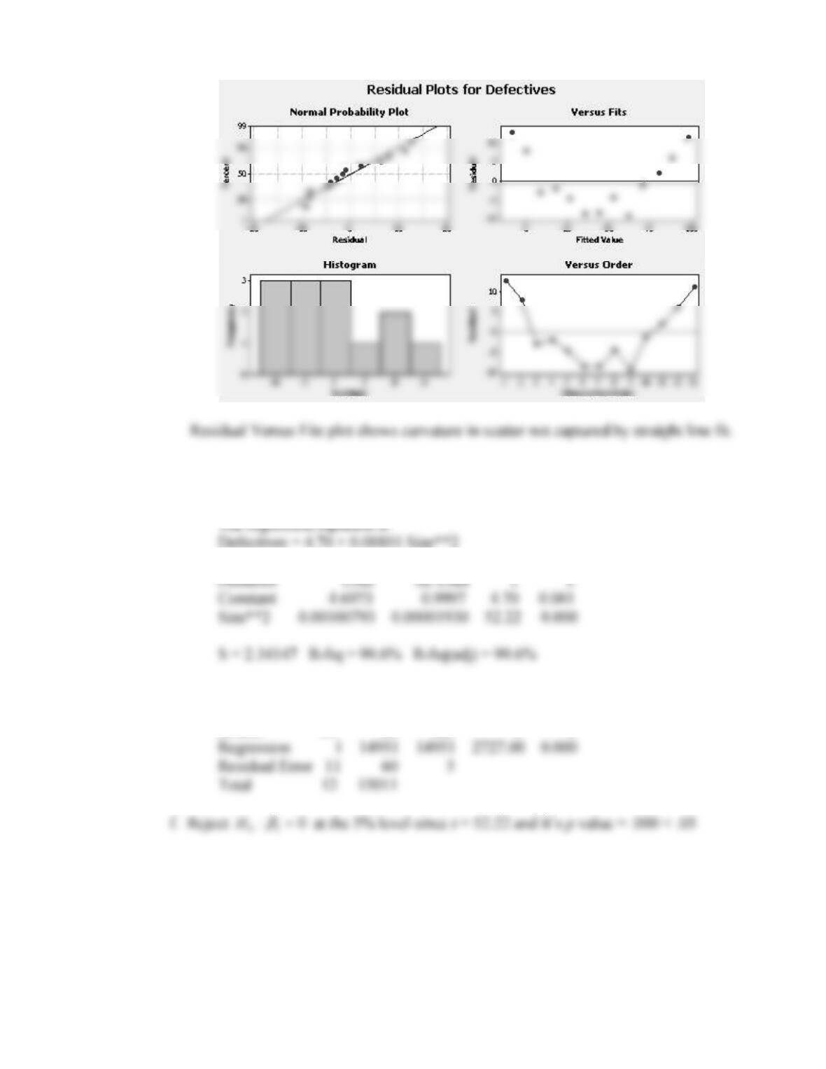
d.
103
e. Model with quadratic term in Batch Size fits well. Results with Size**2 as
predictor variable follow.
Defectives = 4.70 + 0.00101 Size**2
Analysis of Variance
Source DF SS MS F P
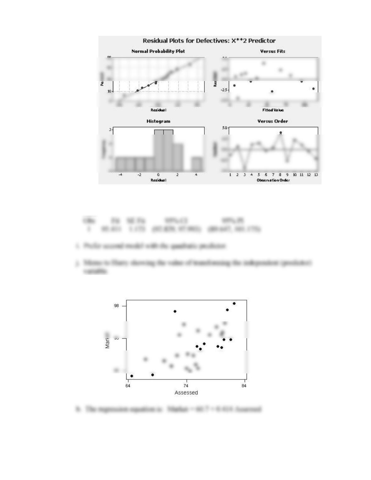
g. Residual plots below indicate an adequate fit.
104
h. Predicted Values for New Observations
New
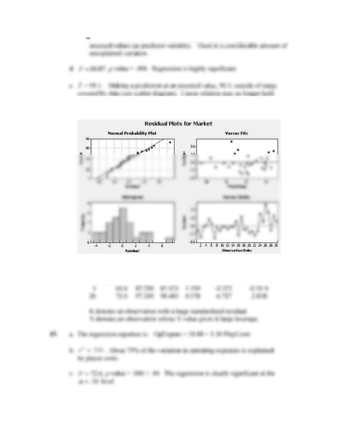
14. a.
105
c. 376.
2
r. About 38% of the variation in market prices is explained by
f. Residual plots follow.
Unusual Observations
Obs Assessed Market Fit SE Fit Residual St Resid
106
d. Coefficient on
X
= player costs is 1.30. Is
2:
10
H
reasonable?
f. Unusual Observations
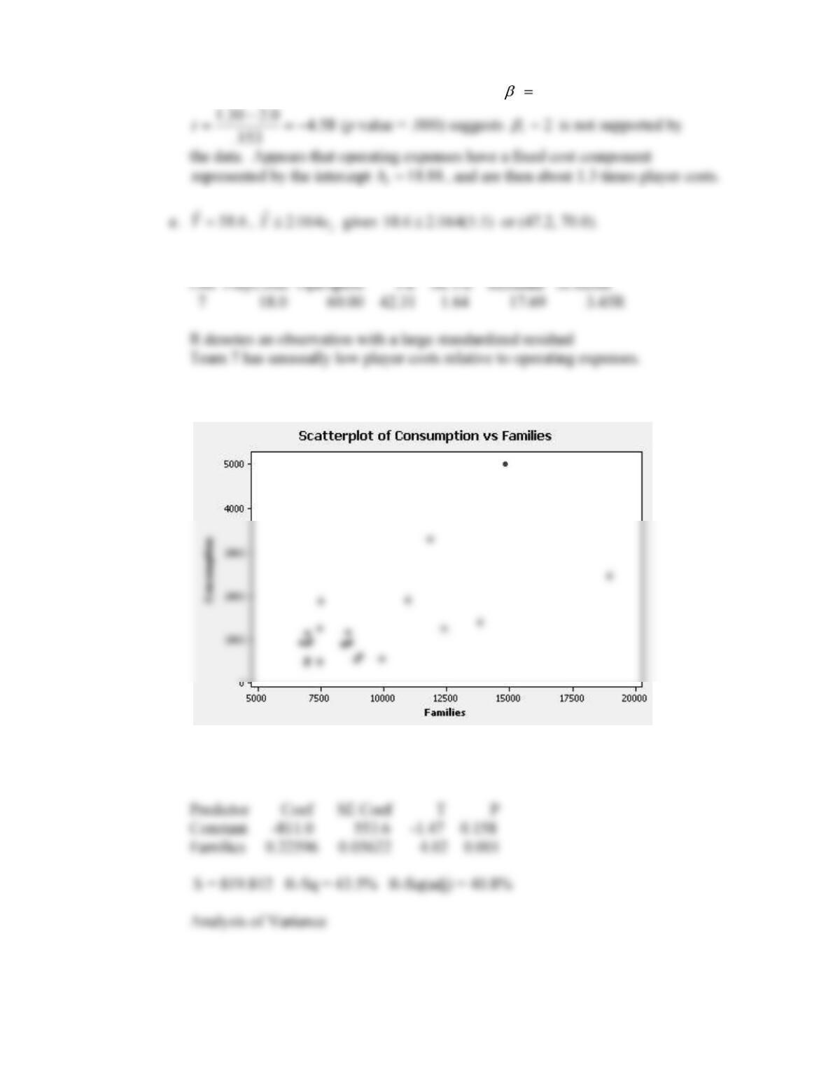
16. a. Scatter diagram follows.
b. The regression equation is
Consumption = – 811 + 0.226 Families