107
Source DF SS MS F P
Regression 1 10855642 10855642 16.15 0.001
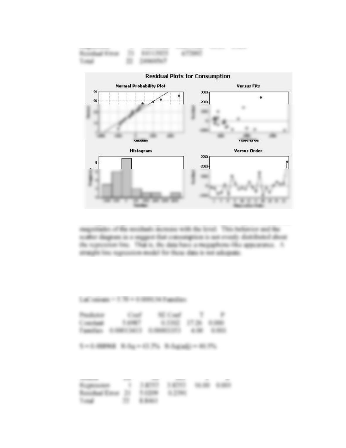
Although the regression is significant, the residual versus fit plot indicates the
c & d. The response variable is converted to the natural log of newsprint consumption
(LnConsum).
The regression equation is
Analysis of Variance
108
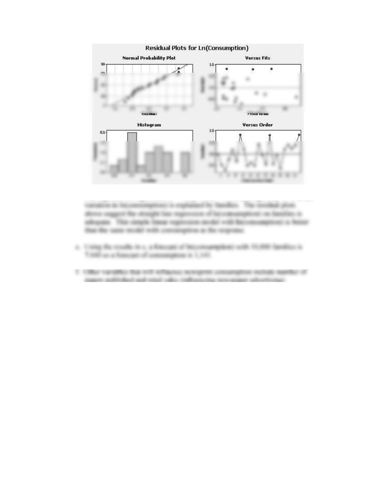
The regression is significant (F = 16, p value = .001) although only 43% of the
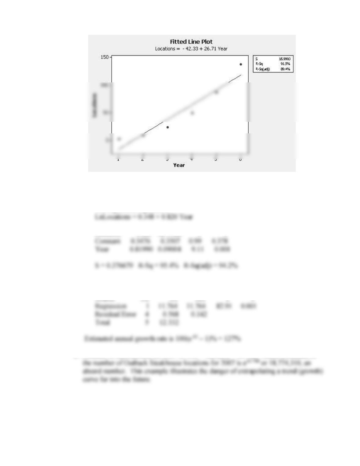
17. a. Can see from fitted line plot below that growth in number of steakhouses is
exponential, not linear.
109
b. The slope of a regression of ln(location) versus year is related to the annual
growth rate.
The regression equation is
Predictor Coef SE Coef T P
Analysis of Variance
c. Forecast of ln(locations) for 2007 is .348 + .820(20) = 16.748. Hence a forecast of
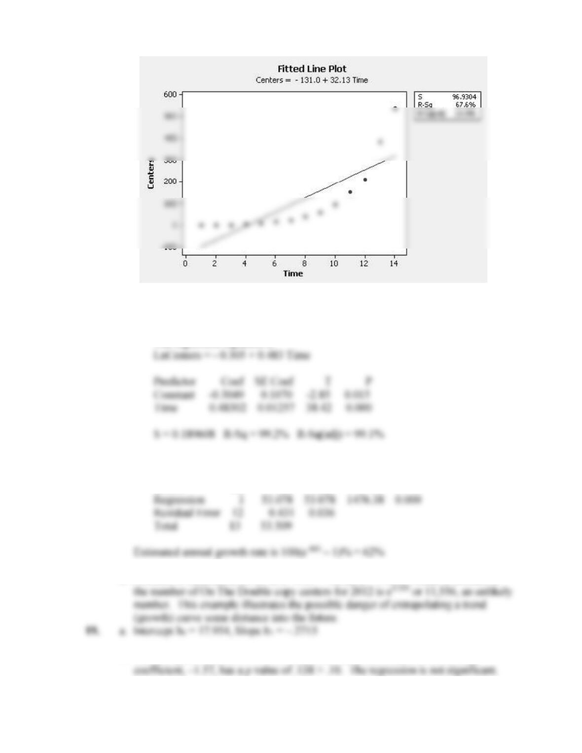
18. a, Can see from fitted line plot below that growth in number of copy centers is
exponential, not linear.
110
b. The slope of a regression of ln(centers) on time (year) is related to the annual
growth rate.
The regression equation is
Analysis of Variance
Source DF SS MS F P
c. Forecast of ln(centers) for 2012 is -.305 + .483(20) = 9.355. Hence a forecast of
b. Cannot reject H0 at the 10% level since the t value associated with the slope
111
20. Deleting Dun and Bradstreet gives the following results:
The regression equation is
Analysis of Variance
Source DF SS MS F P
21. a. The regression equation is
112
Analysis of Variance
Source DF SS MS F P
d. If estimated costs are perfect predictor of actual costs, then
1,0
10 . The
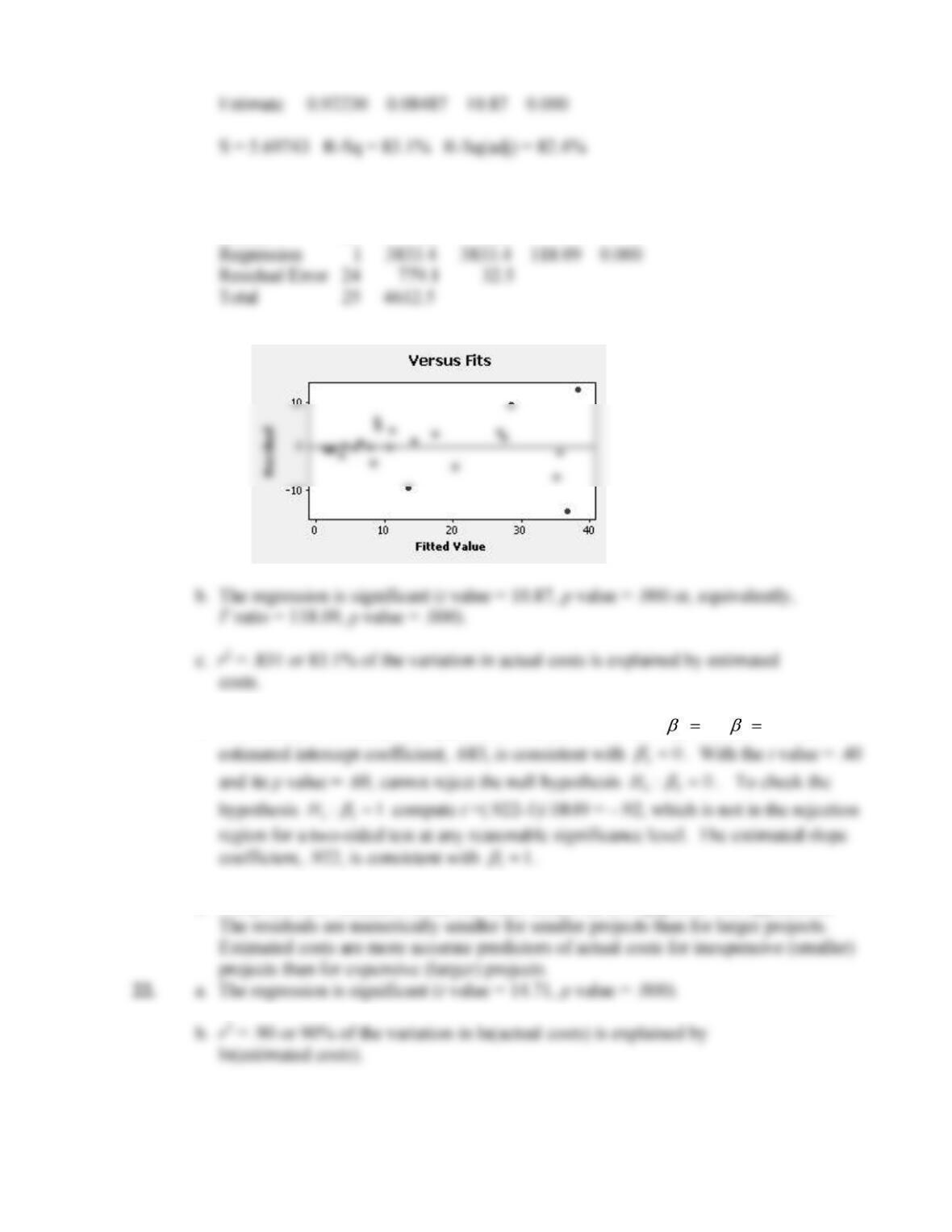
e. The plot of the residuals versus the fitted values has a megaphone-like appearance.
113
CASE 6-1: TIGER TRANSPORT
This case asks students to summarize the analysis in a report to management. We find this a
useful exercise since it requires students to put the application and results of a statistical procedure into
their own words. If they are able to do this, they understand the technique.
This case illustrates the use of regression analysis in a situation where determining a good
regression equation is only the first step. The results must then be priced out in order to
CASE 6-2: BUTCHER PRODUCTS, INC.
3. Since there is a fairly strong relationship between output and deviation from ideal
4. Gene has made a decent start towards finding an effective forecasting tool. However,
CASE 6-3: ACE MANUFACTURING
1. The correlation coefficient is: r = .927. The corresponding t = 8.9 for testing
6. If time and cost are not factors, it might be helpful to take a larger sample to see if these
CASE 6-4: MR. TUX
1. After John uses simple regression analysis to forecast his monthly sales volume, he is
not satisfied with the results. The low r-squared value (56.3%) disappoints him.
3. The idea of serial correlation can be mentioned at this point. The possibility of
autocorrelated residuals can be introduced based on John’s Durbin-Watson statistic.
115
CASE 6-5: CONSUMER CREDIT COUNSELING
1. The correlation of Clients and Stamps = 0.431 and t = 3.24, so relationship is
significant but not very useful.
The regression equation is
Predictor Coef SE Coef T P
Analysis of Variance
Source DF SS MS F P
The regression equation is
Analysis of Variance
Source DF SS MS F P
2. The regression equation is Clients = – 199 + 2.94 BI
results are:
The regression equation is
Analysis of Variance
Source DF SS MS F P
Regressing Clients on the reciprocal of Index produces a little better straight line fit.
Analysis of Variance
3. Actual Forecast Forecast Forecast(RecipIndex predictor)
4. Only if the business activity index could itself be forecasted accurately. Otherwise, it is
117
6. If a good regression equation can be developed in which the changes in the predictor
CASE 6-6: AAA WASHINGTON
1. The four linear regression models are shown below. Both temperature and rainfall are
potential predictor variables.
The regression equation is
The regression equation is
The regression equation is
118
The regression equation is
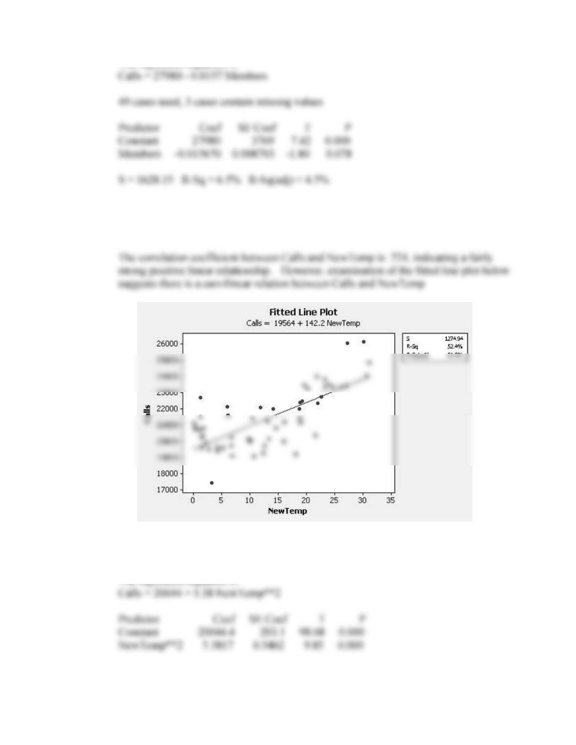
2. & 3. Sixty-five degrees was subtracted from the temperature variable. The variable used
was the absolute value of the temperature with relative zero at 65 degrees Fahrenheit
labeled NewTemp.
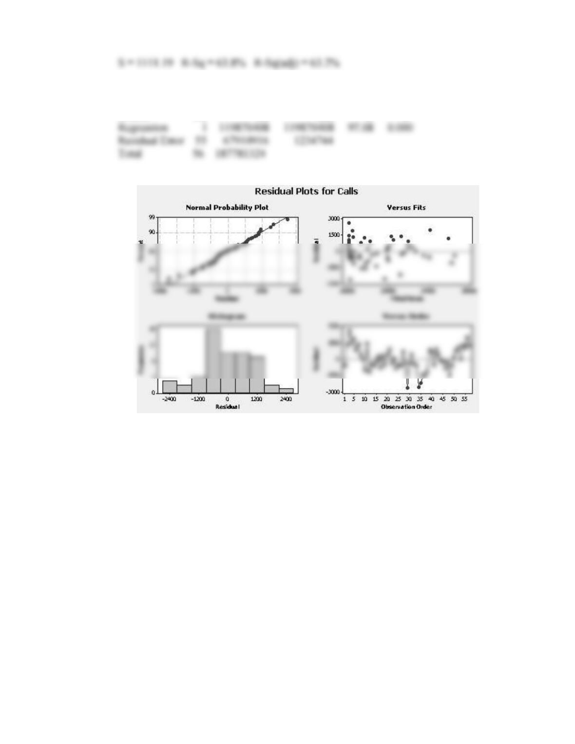
4. A linear regression model with predictor variable NewTemp**2 gives a much
better fit. The residual plots also indicate an adequate fit.
119
Analysis of Variance
Source DF SS MS F P