
Numerical Differentiation, Part I 1
Solutions
Chapter 6 Differentiation and Integration
6.1 Numerical Differentiation, Part I
1. Rework the coefficient of friction problem from the data in Table 6-1 using
a not-a-knot cubic spline interpolant rather than a 10-th degree interpolating
polynomial.
The complete set of not-a-knot cubic spline coefficients is
ajbjcjdj
5.00 0.01459451609473 0.00163632965476 0.00034509300172
12.27 0.03509367276497 0.00488875457180 0.00059664547058
30.10 0.08595968633557 0.01209279518360 0.00145443178964
73.86 0.21092946026941 0.02957214680738 0.00363963236772
The graph below on the left shows that the cubic spline provides a reasonable
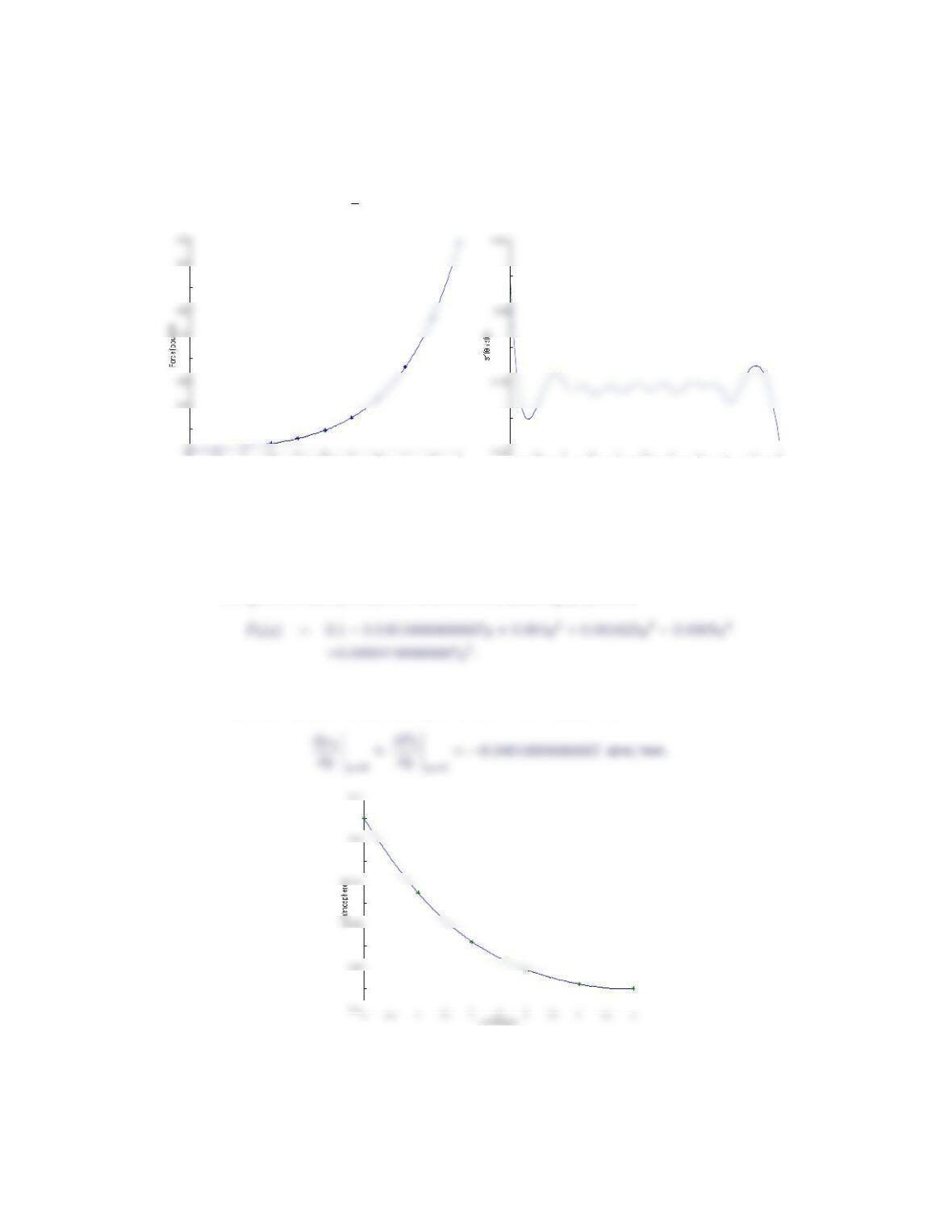
2Section 6.1
regions around θ=π
4,θ= 4πand θ= 5π, where µ= 0.28 to two decimal places.
00.5 11.5 22.5 33.5 44.5 5
50
200
350
! (*“, radians)
00.5 11.5 22.5 33.5 44.5 5
0.284
0.288
0.292
! (*“, radians)
2. Rework the convection mass transfer coefficient problem using a single interpo-
lating polynomial of degree at most 5.
Using all six data points, we obtain the interpolating polynomial
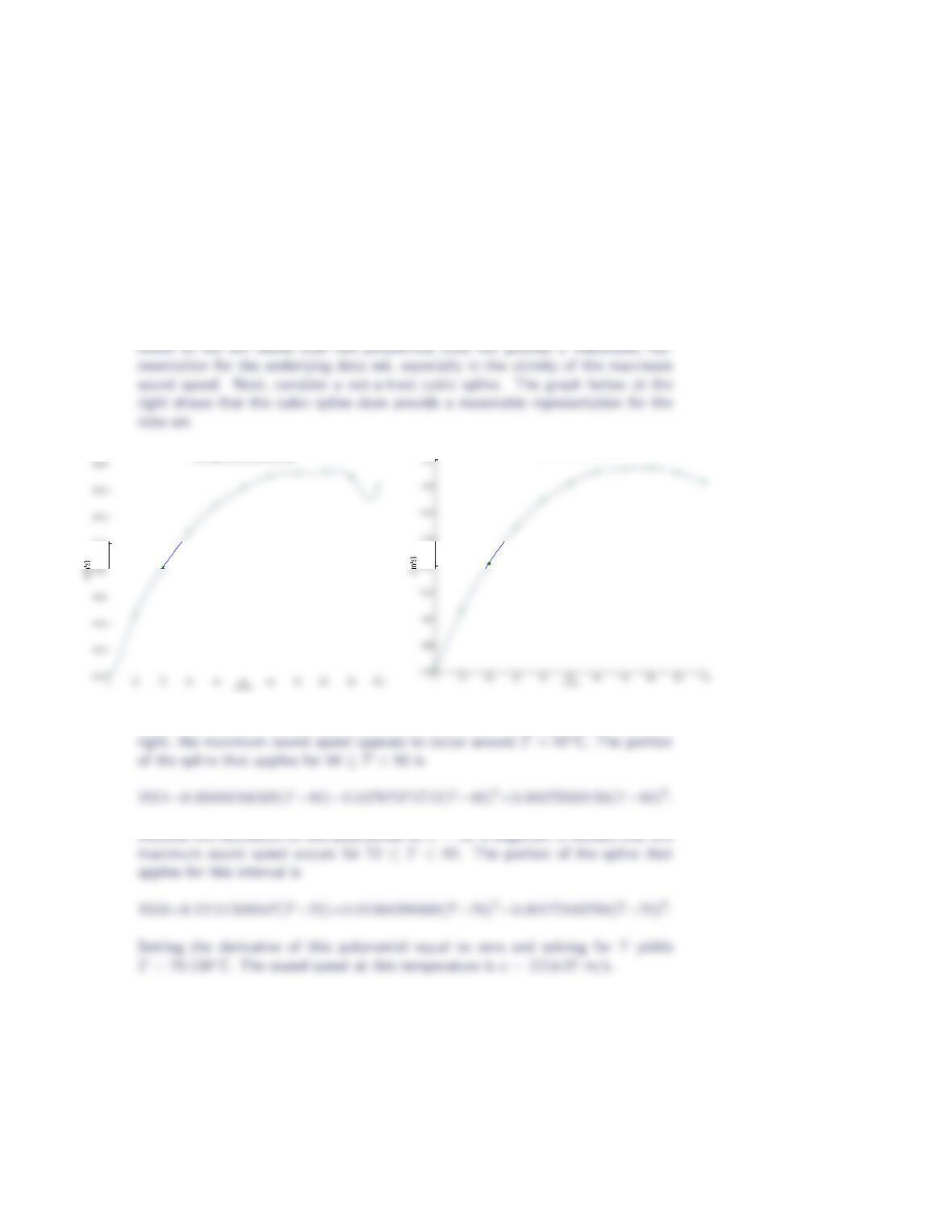
The graph below shows that the interpolating polynomial provides a reasonable
representation for the underlying data set. It then follows that
0.02
0.04
0.06
0.08
0.1
Numerical Differentiation, Part I 3
3. Estimate the temperature, T, at which the sound speed, a, of water is a maxi-
mum. What is the corresponding maximum speed of sound in water?
T(◦C) 0 10 20 30 40 50 60 70 80 90 100
a(m/s) 1402 1447 1482 1509 1529 1542 1551 1553 1554 1550 1543
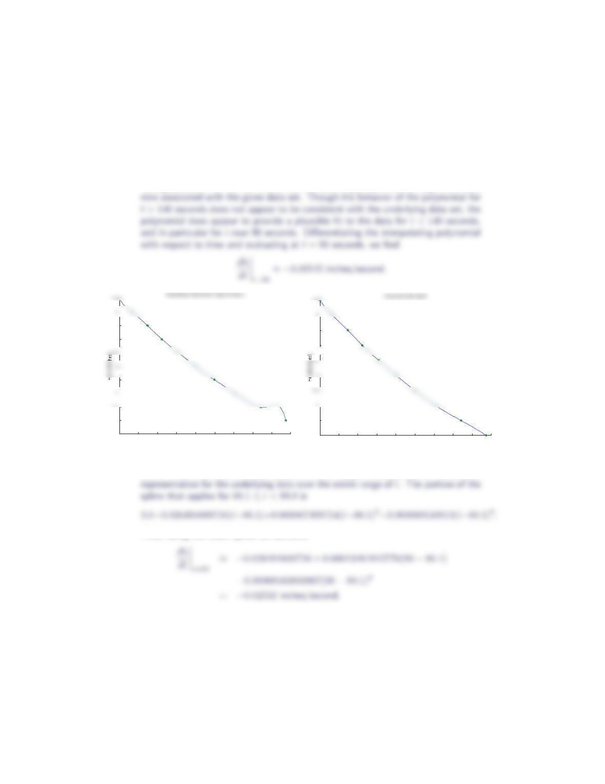
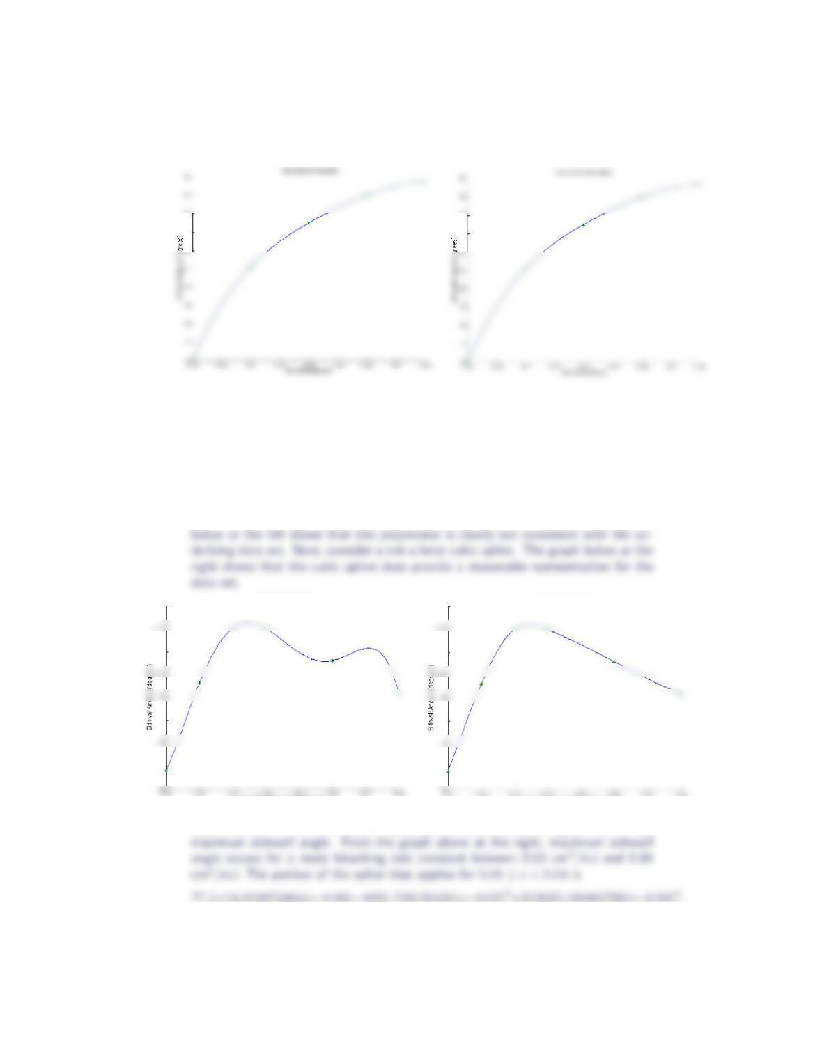
Let’s first try a single interpolating polynomial of degree at most ten. The graph
1500
10th Degree Interpolating Polynomial
1480
Not-a-knot Cubic Spline
Now, let’s determine the maximum sound speed. From the graph above at the
4. The following table provides the height of water in a container as a function of
time during an experiment dealing with Toricelli’s law. Estimate the rate at
which the height of water is changing at t= 90 seconds.
4Section 6.1
time (sec) 0.0 13.2 29.4 44.6 61.8 80.1 99.8 121.5 148.3 174.9
height (inches) 5.5 5.0 4.5 4.0 3.5 3.0 2.5 2.0 1.5 1.0
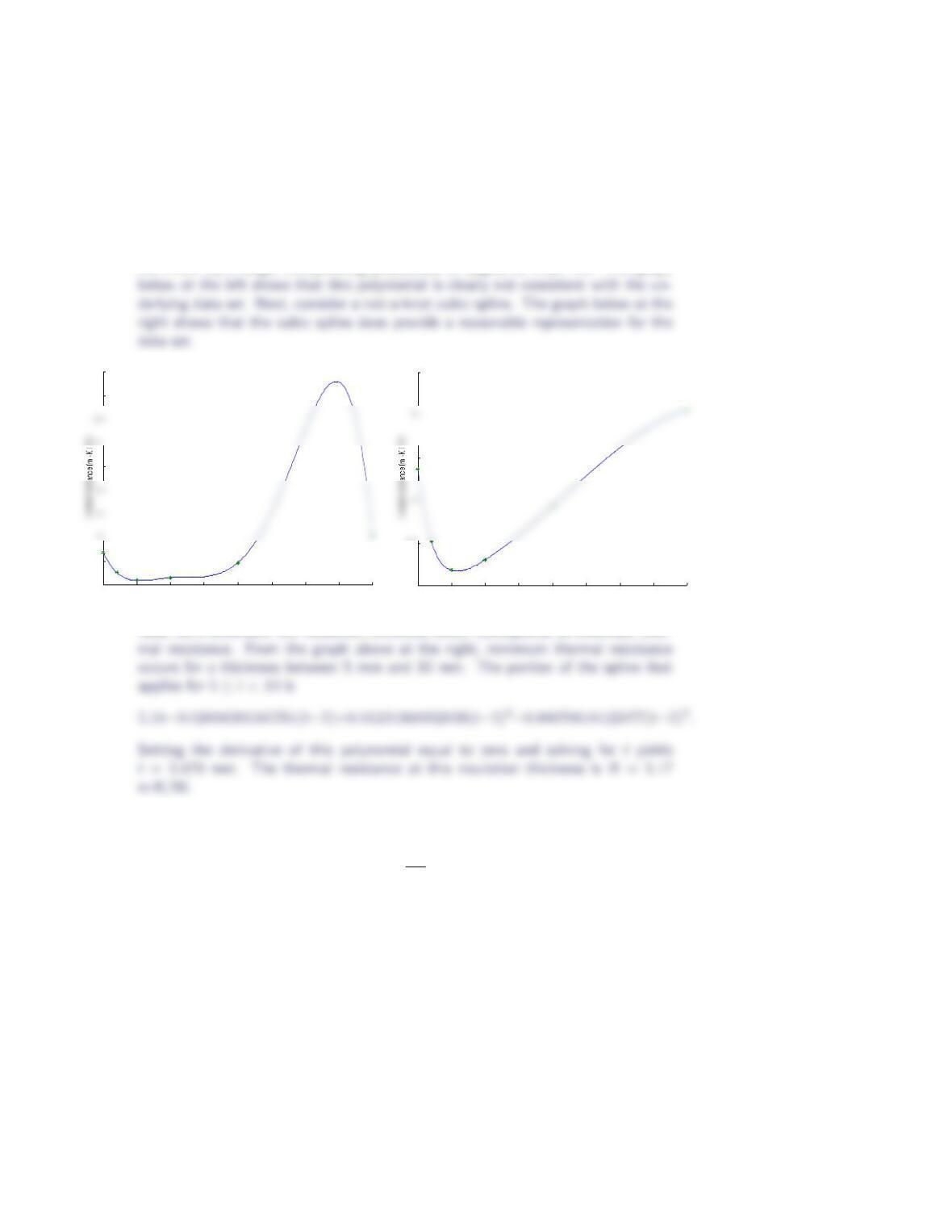
The graph below at the left shows the interpolating polynomial of degree at most
020 40 60 80 100 120 140 160 180
0.5
1
1.5
2.5
4
4.5
Time (seconds)
020 40 60 80 100 120 140 160 180
1
1.5
4.5
5.5
Time (seconds)
Let’s also consider a not-a-knot cubic spline. The graph above on the right shows
that the not-a-knot cubic spline associated with the given data provides a reasonable
Thus, using the cubic spline we estimate
5. The thermal resistance, R, as a function of insulation thickness for a thin-walled
copper tube is provided in the table below. Estimate the insulation thickness
which corresponds to minimum thermal resistance.
Numerical Differentiation, Part I 5
thickness (mm) 0 2 5 10 20 40
thermal resistance R(m·K/W) 6.37 5.52 5.18 5.30 5.93 7.06
Let’s first try a single interpolating polynomial of degree at most five. The graph
0 5 10 15 20 25 30 35 40
5
6
10
13
14
Insulation thickness (mm)
Interpolating Polynomial of Degree at most 5
0 5 10 15 20 25 30 35 40
5
5.5
6.5
7.5
Insulation thickness (mm)
Not-a-knot Cubic Spline
Now, let’s determine the insulation thickness which corresponds to minimum ther-
6. The specific heat at constant pressure, cp, is given by
cp=∂h
∂T p
,
where hdenotes enthalpy and Tdenotes temperature. The parentheses around
the partial derivative are used to indicate the pressure, p, is to be held constant
during this calculation.
The enthalpy of superheated nitrogen as a function of temperature is given in the
table below. Use this data to estimate the specific heat at constant pressure of
superheated nitrogen at a temperature of 200 K. Is the specific heat at constant
pressure of superheated nitrogen constant over the range of temperatures 150
K through 250 K? If not, by how much does it vary?
6Section 6.1
T(K) 100 125 150 175 200
h(kJ/kg) 101.965 128.505 154.779 180.935 207.029
T(K) 225 250 275 300
h(kJ/kg) 233.085 259.122 285.144 311.158
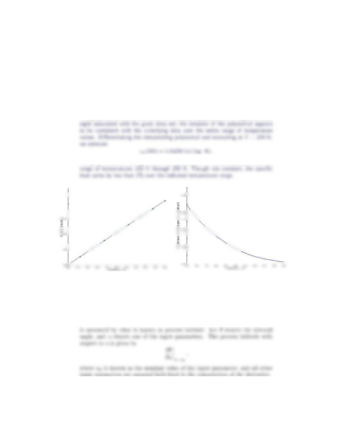
The graph below at the left shows the interpolating polynomial of degree at most
The graph below at the right shows the specific heat at constant pressure over the
300
350
1.042
1.044
1.046
1.048
1.05
7. In optical microlithography one of the most important performance metrics is
the sidewall angle of the photoresist film at the completion of the development
phase. Sidewall angle is a function of many different input parameters, including
exposure energy, development time, thickness of contrast enhancing film and
numerical aperture. Sensitivity of sidewall to any one of these input parameters
in the table below. Estimate the process latitude with respect to film
thickness at a nominal value of 0.20 µm.
film thickness (µm) 0.00 0.10 0.20 0.30 0.40
θ(degrees) 80.7 83.8 85.7 86.2 86.3
(b) Sidewall angle as a function of numerical aperture is given in the table
below. Estimate the process latitude with respect to numerical aperture
at a nominal value of 0.24.
numerical aperture 0.16 0.20 0.24 0.28 0.32
θ(degrees) 76.0 81.1 83.5 85.0 85.7
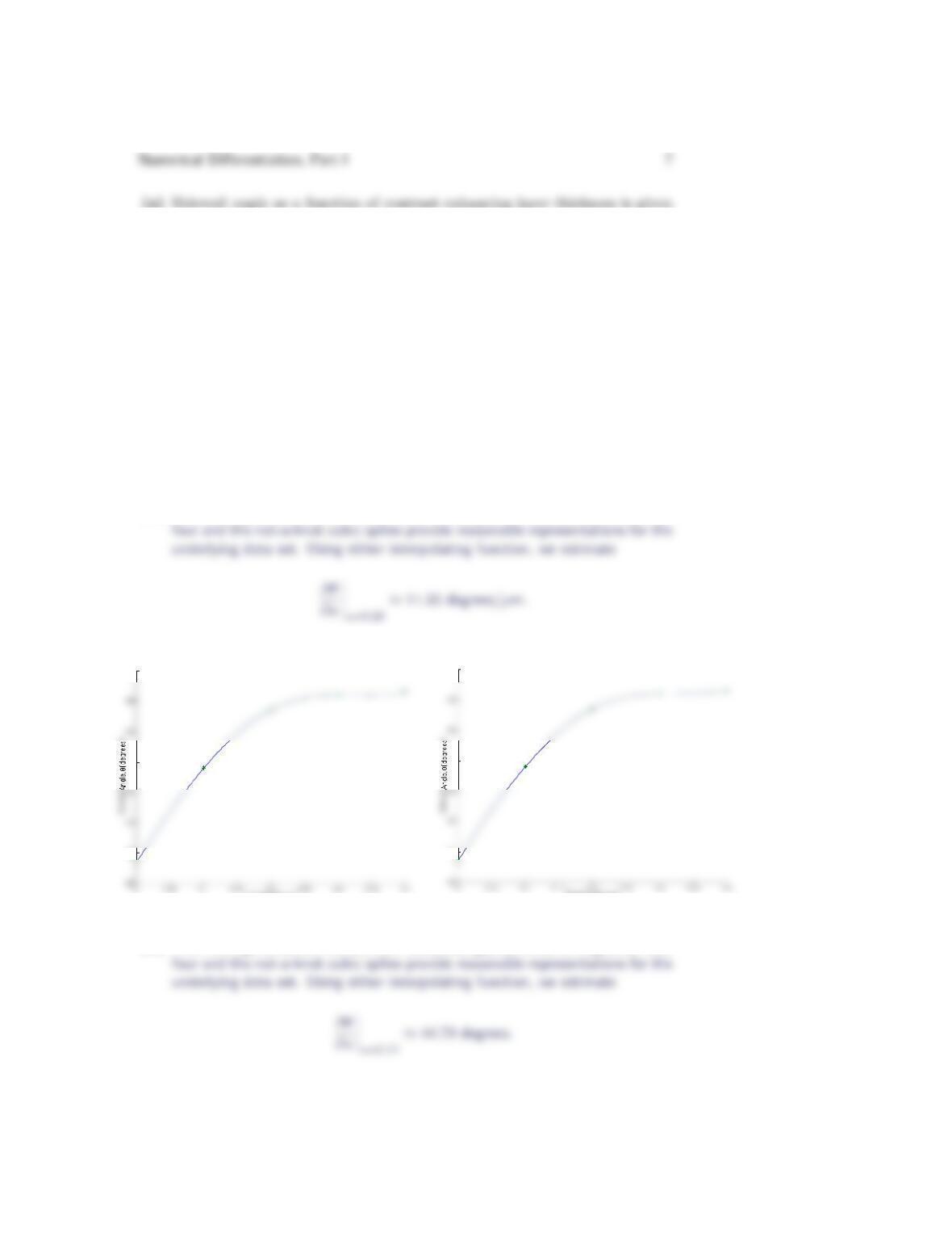
(a) From the figures below, we see that interpolating polynomial of degree at most
81
84
87
Film thickness (µm)
Interpolating Polynomial
81
84
87
Film thickness (µm)
Not-a-knot Cubic Spline
(b) From the figures below, we see that interpolating polynomial of degree at most
8Section 6.1
83
84
83
84
8. Sidewall angle as a function of resist bleaching rate constant is given below.
Estimate the resist bleaching rate constant which gives rise to the maximum
sidewall angle.
bleaching rate constant (cm2/mJ) 0.01 0.02 0.03 0.04 0.06 0.08
θ(degrees) 74.4 76.3 77.5 77.5 76.8 76.1
Let’s first try a single interpolating polynomial of degree at most five. The graph
74.5
75.5
77
78
Bleaching rate constant (cm2 / mJ)
Interpolating Polynomial
0.01 0.02 0.03 0.04 0.05 0.06 0.07 0.08
74.5
75.5
76.5
77
77.5
78
Bleaching rate constant (cm2 / mJ)
Not-a-knot Cubic Spline
Now, let’s determine the resist bleaching rate constant which gives rise to the
Numerical Differentiation, Part I 9
Setting the derivative of this polynomial equal to zero and solving for cyields
c= 0.03429 cm2/mJ. The sidewall angle achieved with this resist bleaching rate
constant is θ= 77.61◦.