6.6 Gaussian Quadrature
1. Approximate the value of each of the following integrals using the two-point
Gaussian quadrature rule (the basic formula, not the composite rule). Verify
that the theoretical error bound holds in each case.
(a) R1
−1e−xdx (b) R1
−1
1
1+x2dx (c) Rπ
0sin xdx (d) R1
0tan−1xdx
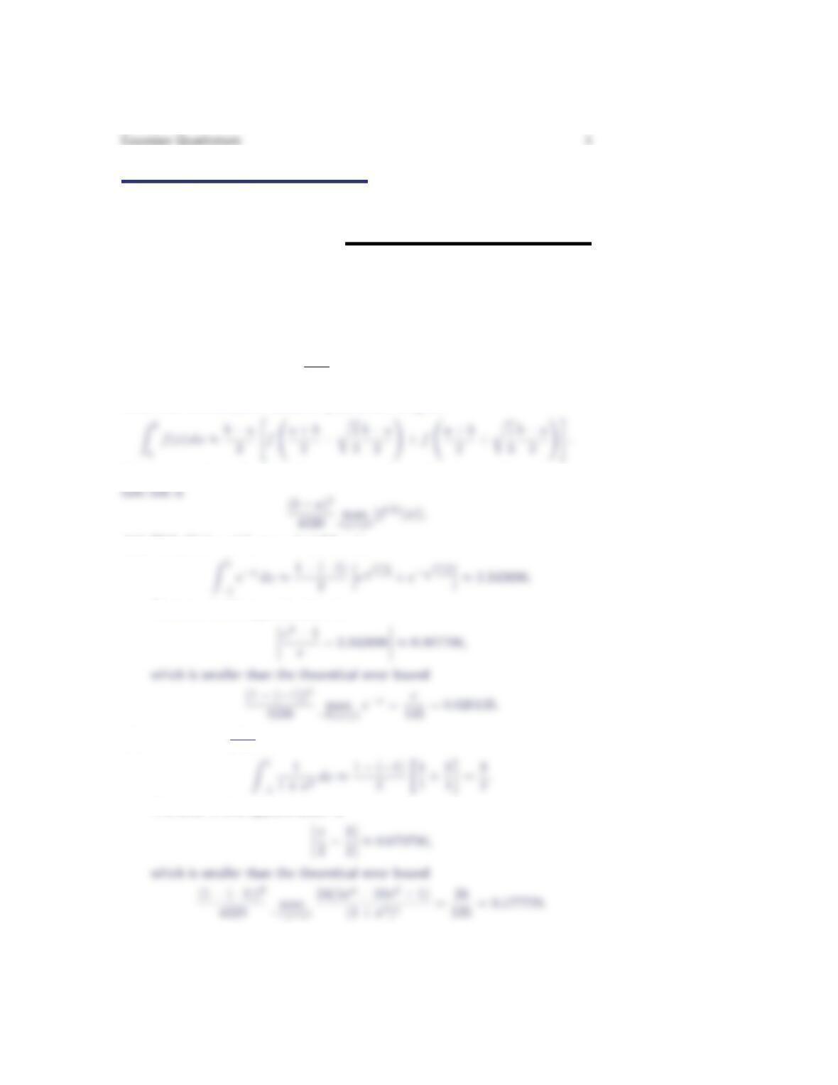
Recall that the two-point Gaussian quadrature rule gives
Moreover, the theoretical error bound associated with the two-point Gaussian quadra-
(a) With f(x) = e−x,a=−1and b= 1,
The error in this approximation is
(b) With f(x) = 1
1+x2,a=−1and b= 1,
The error in this approximation is
2Section 6.6
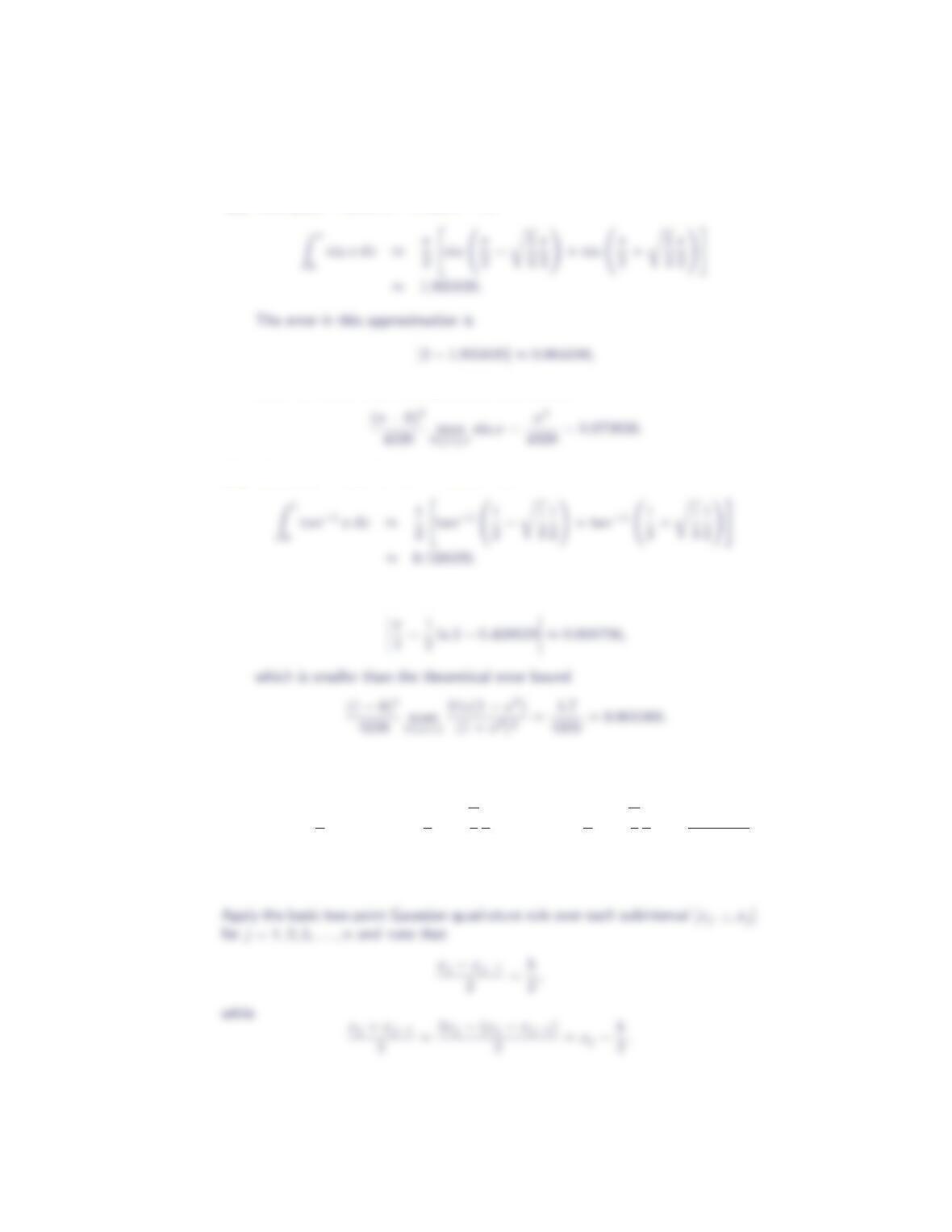
(c) With f(x) = sin x,a= 0 and b=π,
which is smaller than the theoretical error bound
(d) With f(x) = tan−1x,a= 0 and b= 1,
The error in this approximation is
2. Derive the composite two-point Gaussian quadrature rule:
Zb
a
f(x)dx =h
2
n
X
j=1 “f xj−h
2−r1
3
h
2!+f xj−h
2+r1
3
h
2!#+(b−a)h4
4320 f(4)(ξ),
where h= (b−a)/n,xj=a+jh and a < ξ < b.
Gaussian Quadrature 3
Thus,
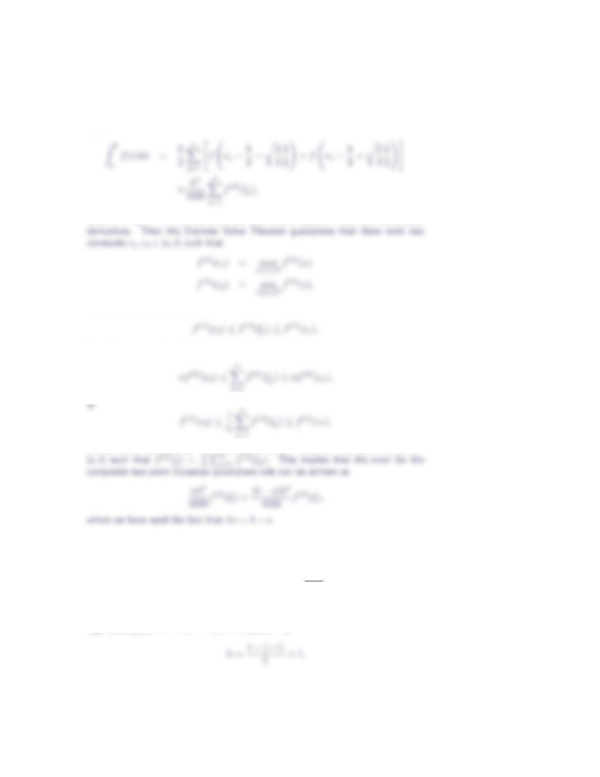
where a < ξj< b. To transform the error term, suppose fhas four continuous
It then follows that for each j
Summing over each subinterval [xj−1, xj], we find that
We can now conclude, by the Intermediate Value Theorem, that there exists ξ∈
3. Approximate the value of each of the following integrals using the composite
two-point Gaussian quadrature rule with the specified number of subintervals.
Verify that the theoretical error bound holds in each case.
(a) R1
−1e−xdx, n = 2 (b) R1
−1
1
1+x2dx, n = 2
(c) Rπ
0sin xdx, n = 3 (d) R1
0tan−1xdx, n = 3
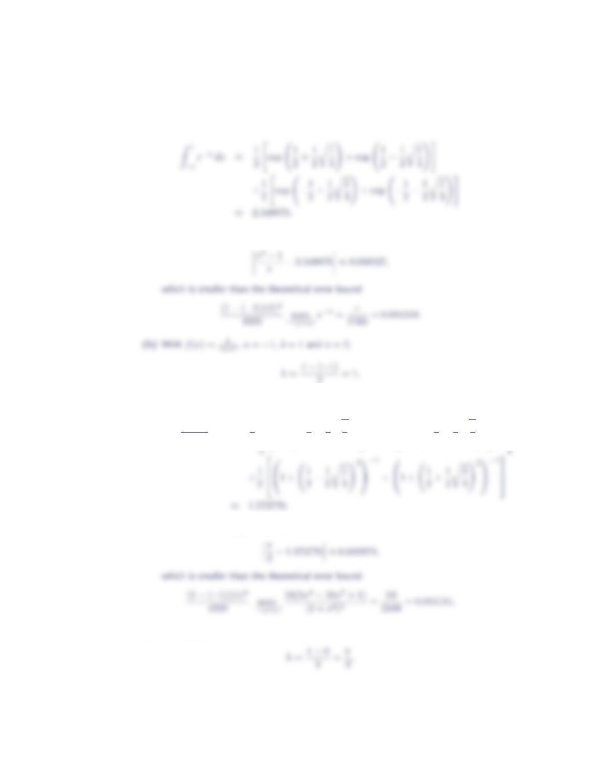
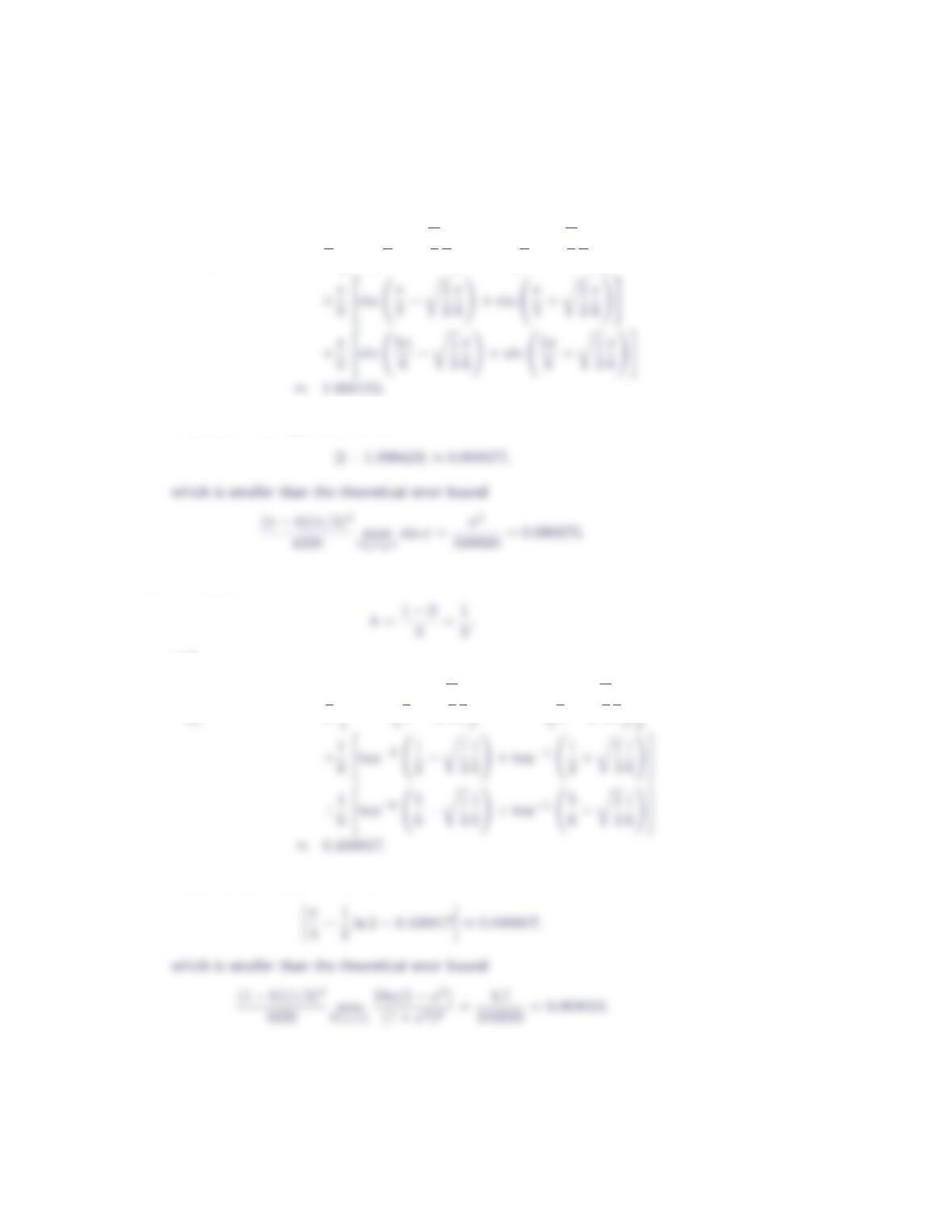
(a) With f(x) = e−x,a=−1,b= 1 and n= 2,
4Section 6.6
and
The error in this approximation is
2= 1,
and
Z1
−1
1
1 + x2dx ≈1
2
1 + −1
2−1
2r1
3!2
−1
+
1 + −1
2+1
2r1
3!2
−1
The error in this approximation is
(c) With f(x) = sin x,a= 0,b=π, and n= 3,
Gaussian Quadrature 5
and
Zπ
0
sin x dx ≈π
6“sin π
6−r1
3
π
6!+ sin π
6+r1
3
π
6!#
The error in this approximation is
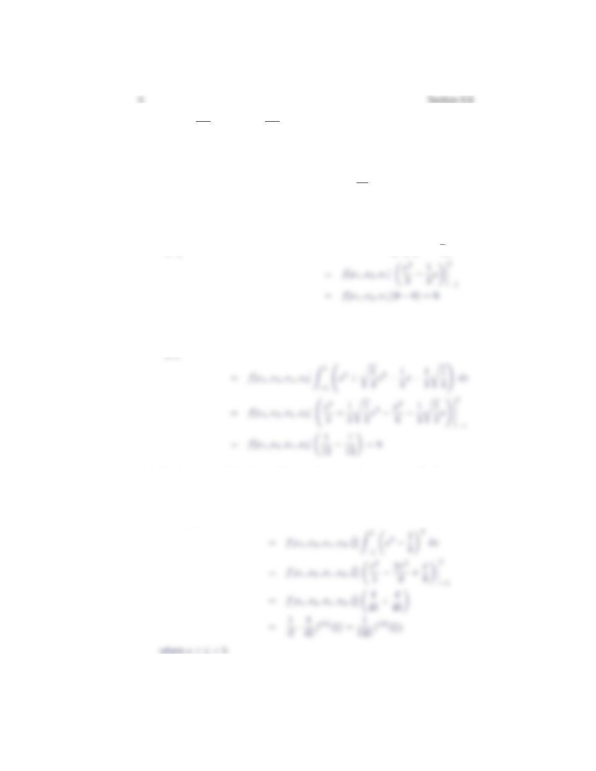
(d) With f(x) = tan−1x,a= 0,b= 1, and n= 3,
and
Z1
tan−1x dx ≈1
6“tan−1 1
6−r1
3
1
6!+ tan−1 1
6+r1
3
1
6!#
The error in this approximation is
4. Let x1=−p1/3 and x2=p1/3. Show that
(a) R1
−1f[x1, x2, x1](x−x1)(x−x2)dx = 0;
(b) R1
−1f[x1, x2, x1, x2](x−x1)2(x−x2)dx = 0; and
(c) R1
−1f[x1, x2, x1, x2, x](x−x1)2(x−x2)2dx =1
135 f(4)(ξ), where a < ξ < b.
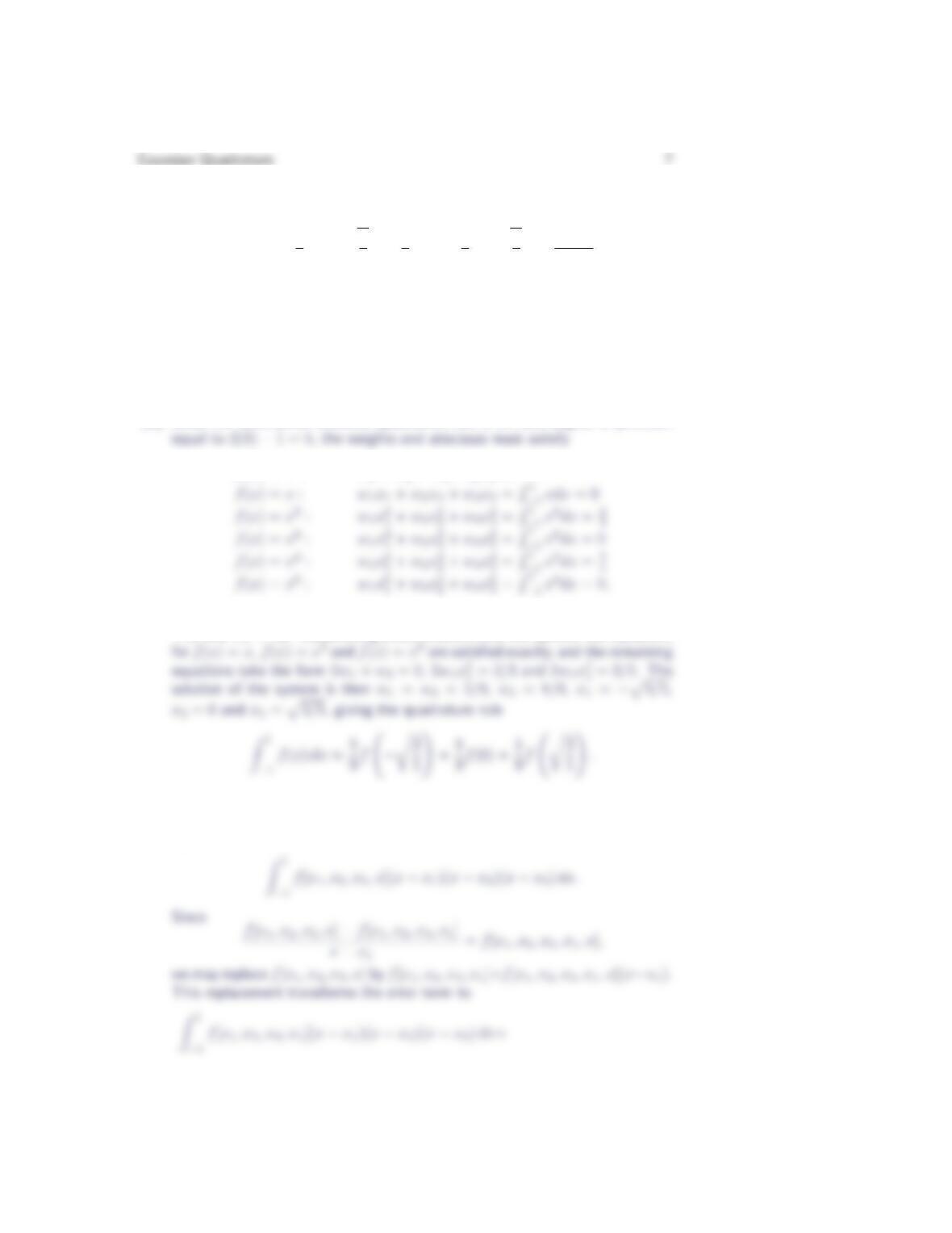
(a)
Z1
f[x1, x2, x1](x−x1)(x−x2)dx =f[x1, x2, x1]Z1
3dx
(b)
Z1
f[x1, x2, x1, x2](x−x1)2(x−x2)dx
(c) By the weighted Mean Value Theorem for Integrals, there exsits ˆ
ξ∈[a, b]such
that
Z1
−1
f[x1, x2, x1, x2, x](x−x1)2(x−x2)2dx
5. (a) Derive the three-point Gaussian quadrature rule
Z1
−1
f(x)dx =5
9f −r3
5!+8
9f(0) + 5
9f r3
5!+1
15750f(6)(ξ),
where −1< ξ < 1.
(b) Convert the quadrature rule from part (a) to the general integration inter-
val [a, b].
(c) Derive the composite three-point Gaussian quadrature rule. (Note: The
rate of convergence should be O(h6).)
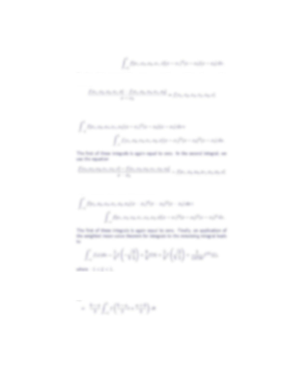
(a) Since the three-point Gaussian quadrature rule is to have degree of precision
f(x) = 1 : w1+w2+w3=R1
The symmetry of the integration interval about zero suggests x2= 0,x3=
−x1and w1=w3. Substituting these relations into the system, the equations
To determine the error term associated with the three-point Gaussian quadra-
ture rule, we start from
8Section 6.6
The first of these integrals is equal to zero. In the second integral, we use the
equation
to replace f[x1, x2, x3, x1, x]by f[x1, x2, x3, x1, x2]+f[x1, x2, x3, x1, x2, x](x−
x2). Now the error term takes the form
to replace f[x1, x2, x3, x1, x2, x]by f[x1, x2, x3, x1, x2, x3]+f[x1, x2, x3, x1, x2, x3, x](x−
x3). The error term then takes the form
(b) Converting this rule back to the more general integration interval [a, b]pro-
duces
Zb
f(x)dx
Gaussian Quadrature 9
=b−a
2“5
9f a+b
2−r3
5
b−a
2!+8
9fa+b
2+5
9f a+b
2+r3
5
b−a
2!
(c) Apply the basic three-point Gaussian quadrature rule over each subinterval
[xj−1, xj]for j= 1,2,3, . . . , n and note that
where a < ξj< b. To transform the error term, suppose fhas six continuous
or
f(6)(c2)≤1
n
n
X
j=1
f(6)(ξj)≤f(6)(c1).
6. Use the three-point Gaussian quadrature rule to approximate the value of the
definite integral R2
1
1
xdx. What is the absolute error in this approximation?
With f(x) = 1
x,a= 1 and b= 2,
7. Repeat Exercise 1 using the three-point Gaussian quadrature rule.
Recall that the three-point Gaussian quadrature rule gives
Gaussian Quadrature 11
(b) With f(x) = 1
1+x2,a=−1and b= 1,
(c) With f(x) = sin x,a= 0 and b=π,
(d) With f(x) = tan−1x,a= 0 and b= 1,
8. Repeat Exercise 3 using the composite three-point Gaussian quadrature rule.
(a) With f(x) = e−x,a=−1,b= 1, and n= 2,
h=1−(−1)
2= 1,
and
(b) With f(x) = 1
1+x2,a=−1,b= 1, and n= 2,
The error in this approximation is
Gaussian Quadrature 13
(c) With f(x) = sin x,a= 0,b=π, and n= 3,
and
Zπ
sin x dx ≈π
6“5
9sin π
6−r3
5
π
6!+8
9sin π
6+5
9sin π
6+r1
3
π
6!#
The error in this approximation is
which is smaller than the theoretical error bound
(d) With f(x) = tan−1x,a= 0,b= 1, and n= 3,
and
Z1
0
tan−1x dx ≈1
6“5
9tan−1 1
6−r3
5
1
6!+8
9tan−11
6+5
9tan−1 1
6+r3
5
1
6!#
The error in this approximation is
14 Section 6.6
In Exercises 9 – 16, verify that the composite two-point Gaussian quadrature
rule has rate of convergence O(h4) and the composite three-point Gaussian
quadrature rule has rate of convergence O(h6) by approximating the value of
the indicated definite integral.
9. R1
0√1 + x3dx
Consider the definite integral
The table below lists composite two-point Gaussian quadrature rule approximations
and composite three-point Gaussian quadrature rule approximations to I(f)for
several values of h. Observe that the ratios
hGQ2h
GQ2h−GQ2h/2
GQ2h/2−GQ2h/4GQ3h
GQ3h−GQ3h/2
GQ3h/2−GQ3h/4
1/2 1.11150449274959 16.085 1.11144794625511 15.537
10. Rπ
0sin xdx
Consider the definite integral
I(f) = Zπ
0
sin x dx.
Gaussian Quadrature 15
hGQ2h|e2h/eh|GQ3h|e2h/eh|
π/21.99694522680823 2.00001624311100
11. R2
1
1
xdx
Consider the definite integral
I(f) = Z2
1
1
xdx.
The table below lists composite two-point Gaussian quadrature rule approximations
hGQ2h|e2h/eh|GQ3h|e2h/eh|
1/2 0.693076638282120 0.693146495829060
12. R1
0e−xdx
Consider the definite integral
16 Section 6.6
several values of h. Observe that the ratio |e2h/eh|for the composite two-point
hGQ2h|e2h/eh|GQ3h|e2h/eh|
1/2 0.632111485668375 0.632120553970708
13. R1
0tan−1xdx
Consider the definite integral
The table below lists composite two-point Gaussian quadrature rule approximations
and composite three-point Gaussian quadrature rule approximations to I(f)for
hGQ2h|e2h/eh|GQ3h|e2h/eh|
1/2 0.438784449480132 0.438824858188918
14. R2
1
sin x
xdx
Consider the definite integral
Gaussian Quadrature 17
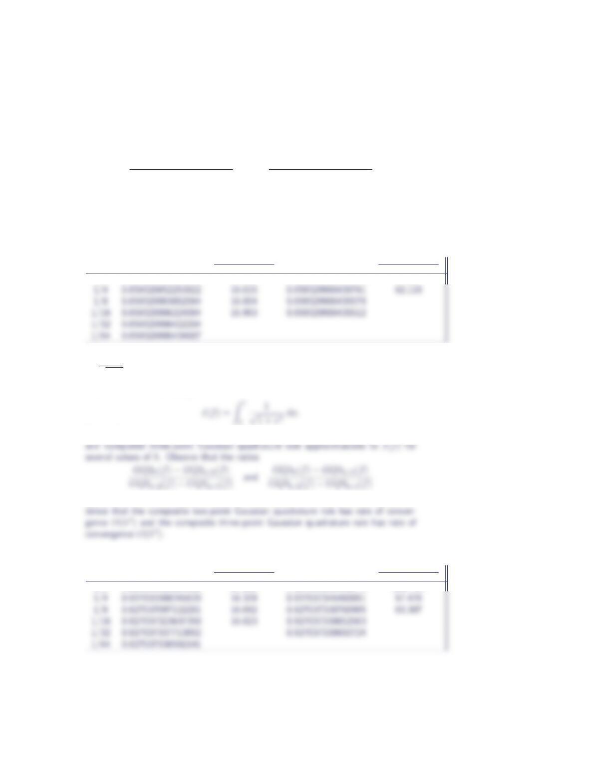
The table below lists composite two-point Gaussian quadrature rule approximations
and composite three-point Gaussian quadrature rule approximations to I(f)for
several values of h. Observe that the ratios
GQ2h(f)−GQ2h/2(f)
GQ2h/2(f)−GQ2h/4(f)and GQ3h(f)−GQ3h/2(f)
GQ3h/2(f)−GQ3h/4(f)
approach 16 and 64, respectively as his decreased. This provides numerical evi-
dence that the composite two-point Gaussian quadrature rule has rate of conver-
gence O(h4)and the composite three-point Gaussian quadrature rule has rate of
convergence O(h6).
hGQ2h
GQ2h−GQ2h/2
GQ2h/2−GQ2h/4GQ3h
GQ3h−GQ3h/2
GQ3h/2−GQ3h/4
1/2 0.659329036510860 16.059 0.659329906707278 64.281
15. R1
0
1
√1+x4dx
Consider the definite integral
The table below lists composite two-point Gaussian quadrature rule approximations
approach 16 and 64, respectively as his decreased. This provides numerical evi-
hGQ2h
GQ2h−GQ2h/2
GQ2h/2−GQ2h/4GQ3h
GQ3h−GQ3h/2
GQ3h/2−GQ3h/4
1/2 0.926954926629315 21.215 0.927039130551673 266.763