1
CHAPTER 6
Problem 6.1
Determine the deformation response u(t) for 0 ≤ t ≤
15 sec for an SDF system with natural period Tn = 2
Solution
1. Initial calculation.
99803.0cos t
Substituting these in Table 5.2.1 of the book with
1
m and 2
n
k
gives
99803.0
A B = 0.019987
2. Apply recurrence Eq. (5.2.5).
3. Plot response history.
Table P6.1a: Numerical solution using piece-wise linear interpolation of excitation
i
t i
p i
Cp 1i
Dp i
uB i
u
i
Au i
u
0.0200 –2.4318 –0.0003 –0.0001 –0.0005 –0.0243 –0.0002 –0.0002
0.0600 –0.3821 –0.0001 –0.0001 –0.0016 –0.0801 –0.0025 –0.0025
0.1000 –2.9259 –0.0004 –0.0003 –0.0029 –0.1445 –0.0067 –0.0067
0.1400 –2.6325 –0.0004 –0.0001 –-0.0056 –0.2798 –0.0152 –0.0152
Table P6.1b: Numerical solution using piece-wise linear interpolation of excitation
i
t i
p i
pC 1
i
pD i
uB
i
u
i
uA i
u
0.0200 –2.4318 –0.0243 –0.0140 –0.0243 0.0243 0.0000 –0.0002
0.0600 –0.3821 –0.0038 –0.0165 –0.0799 –0.0801 0.0005 –0.0025
0.1000 –2.9259 –0.0292 –0.0419 –0.1442 –0.1445 0.0013 –0.0067
0.1400 –2.6325 –0.0263 –0.0107 –0.2793 –0.2798 0.0030 –0.0152
0.1800 0.4941 0.0049 –0.0142 –0.3136 –0.3142 0.0054 –0.0275
2
Problem 6.2
Solve Problem 6.1 for ζ = 5%.
Solution
1. Initial calculation.
99686.0
t
n
e
062712.0sin t
D
Substituting these in Table 5.2.1 of the textbook with
1
m and 2
n
k
gives
99803.0
A B = 0.019924
2. Apply recurrence Eq. (5.2.5).
3. Plot response history.
i
t i
p i
Cp 1i
Dp i
uB i
u
i
Au i
u
0.0200 –2.4318 –0.0003 –0.0001 –0.0005 –0.0243 –0.0002 –0.0002
0.0600 –0.3821 –0.0001 –0.0001 –0.0016 –0.0793 –0.0025 –0.0025
0.1000 –2.9259 –0.0004 –0.0003 –0.0028 –0.1424 –0.0066 –0.0066
0.1400 –2.6325 –0.0004 –0.0001 –0.0055 –0.2752 –0.0150 –0.0150
0.1800 0.4941 0.0001 –0.0001 –0.0061 –0.3059 –0.0270 –0.0271
0.2000 –1.4205 –0.0002 –0.0002 –0.0061 –0.3073 –0.0331 –0.0331
Table P6.2b: Numerical solution using piece-wise linear interpolation of excitation
i
t i
p i
pC 1
i
pD i
uB
i
u
i
uA i
u
0.0200 –2.4318 –0.0242 –0.0140 –0.0241 –0.0243 0.0000 –0.0002
0.0600 –0.3821 –0.0038 –0.0165 –0.0787 –0.0793 0.0005 –0.0025
0.1000 –2.9259 –0.0291 –0.0419 –0.1412 –0.1424 0.0013 –0.0066
0.1400 –2.6325 –0.0262 –0.0107 –0.2729 –0.2752 0.0030 –0.0150
0.1800 0.4941 0.0049 –0.0142 –0.3034 –0.3059 0.0053 –0.0271
Table P6.2a: Numerical solution using piece-wise linear interpolation of excitation
3
Problem 6.3
Solve Problem 6.2 by the central difference method.
Solution
We will solve this problem by the central difference
00
00
uu
nn
Substituting these into Eqs. (1.1)–(1.5) in Table 5.3.1
of the book gives
01
00
ˆ2507.9 2942.1 4990.1
uu
kab
2. Calculations for each time step.
3. Plot response history.
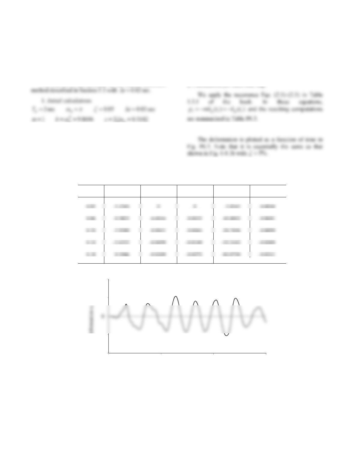
Table P6.3: Numerical solution by central difference method
i
t i
p 1i
u i
u i
p
ˆ 1i
u
0 0 0 0 0 0
0.04 –1.4065 0 –0.0010 –6.2503 –0.0025
0.08 –1.6538 –0.0025 –0.0041 –16.1372 –0.0064
0.12 –4.2002 –0.0064 –0.0099 –37.3192 –0.0149
0.16 –1.0703 –0.0149 –0.0209 –68.1395 –0.0272
0.20 –1.4220 –0.0272 –0.0331 –99.0081 –0.0395
-10
10
0 5 10 15
Deformation u, in.
Time, sec
Figure P6.3
4
Problem 6.4
Derive equations for the deformation, pseudo-velocity,
and pseudo-acceleration response spectra for ground
ζ = 0 and 10%.
Solution
We have solved a related equation:
ut ht met
D
t
D
n
() () sin
1
(b)
ut uet
go
D
t
D
n
()
sin
(c)
The maximum occurs at
and the maximum response is
sin
Do
t12 (g)
1
Substituting Eqs. (f) and (g) in Eq. (e) and using
Dn
12 gives
Response spectra:
VTD
n
2
For
0,
go
go
5
8
10
Tn
0246810
0
0.5
1.5
Tn
go
0246810
0
0.5
2
Tn
6
Problem 6.5
An SDF undamped system is subjected to ground motion
(b) Determine the deformation response spectrum for this
(c) Determine the pseudo-velocity response spectrum for
this excitation with td = 0.5 sec by plotting V/ݑሶ go as a
function of fn = 1/Tn.
Figure P6.5
Solution
1. Determine response to the first impulse.
The ground motion impulse can be represented by the
1() sin
go
n
n
ut t
(a)
2. Determine response to second impulse.
3. Determine response to both impulses.
( ) [sin sin ( )]
go
nnd
n
u
ut t t t
4. Plot displacement response.
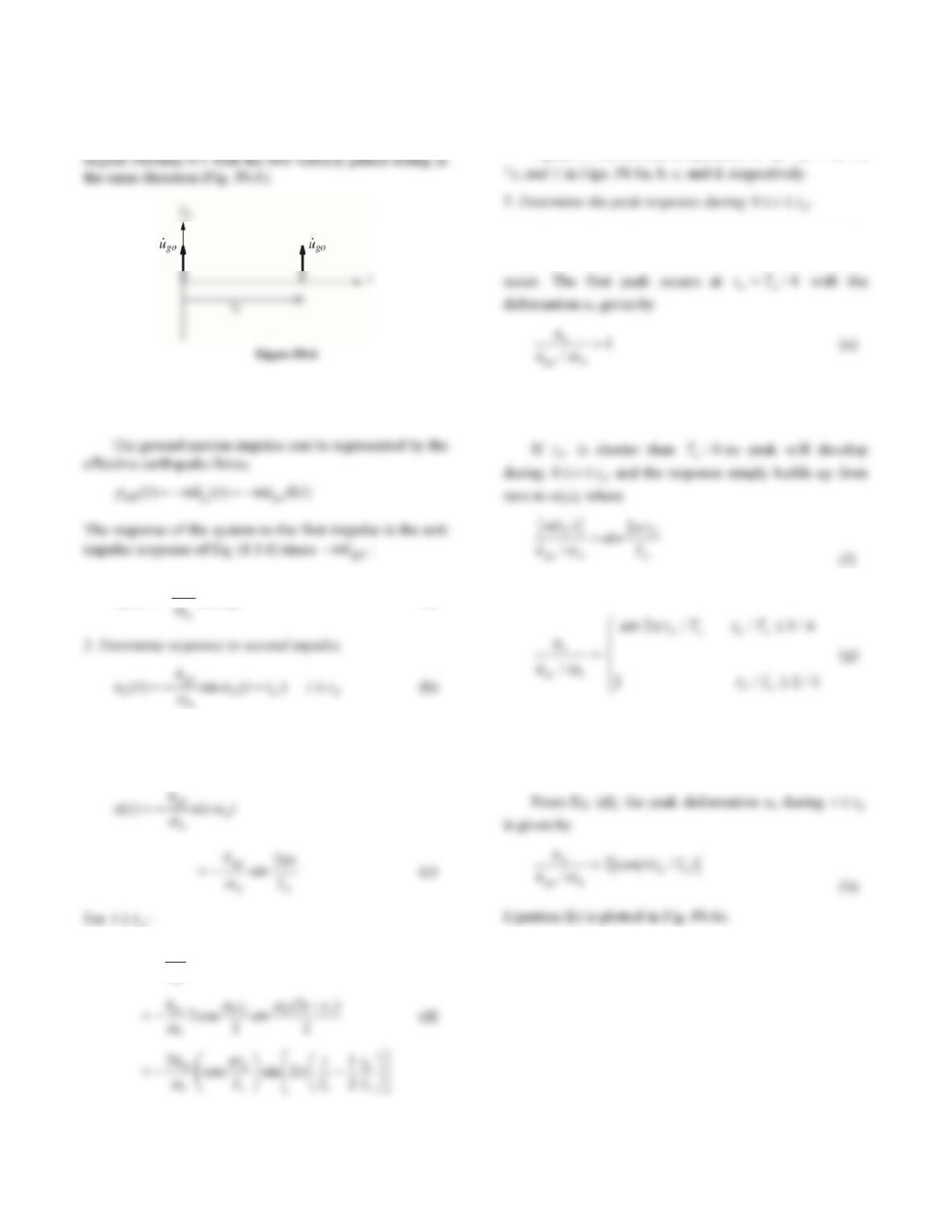
5. Determine the peak response during 0
tt
d.
The number of peaks in u(t) depend on tT
dn
/; the
Thus td must be longer than Tn/4for at least one peak
to develop during 0
tt
d.
If td is shorter than Tn/4no peak will develop
during 0
tt
d and the response simply builds up from
zero to u(td), where
/1/1/4
dn dn
o
go n
dn
u
utT
(g)
From Eq. (d), the peak deformation uo during tt
d
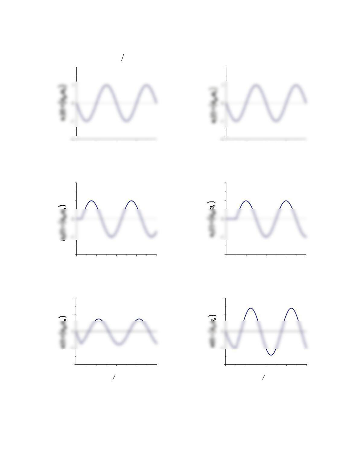
7
00.511.52
2
tT
dn
18
First impulse
00.511.52
2
tT
dn
14
First impulse
00.511.52
-2
1
2
Second impulse
00.511.52
-2
1
2Second impulse
0 0.5 1 1.5 2
-2
-1
1
2
tT
n
Both impulses
utu
0 0.5 1 1.5 2
-2
-1
1
2
tT
n
Both impulses
Figure P6.5a Figure P6.5b
/18
dn
tT /4
dn
tT
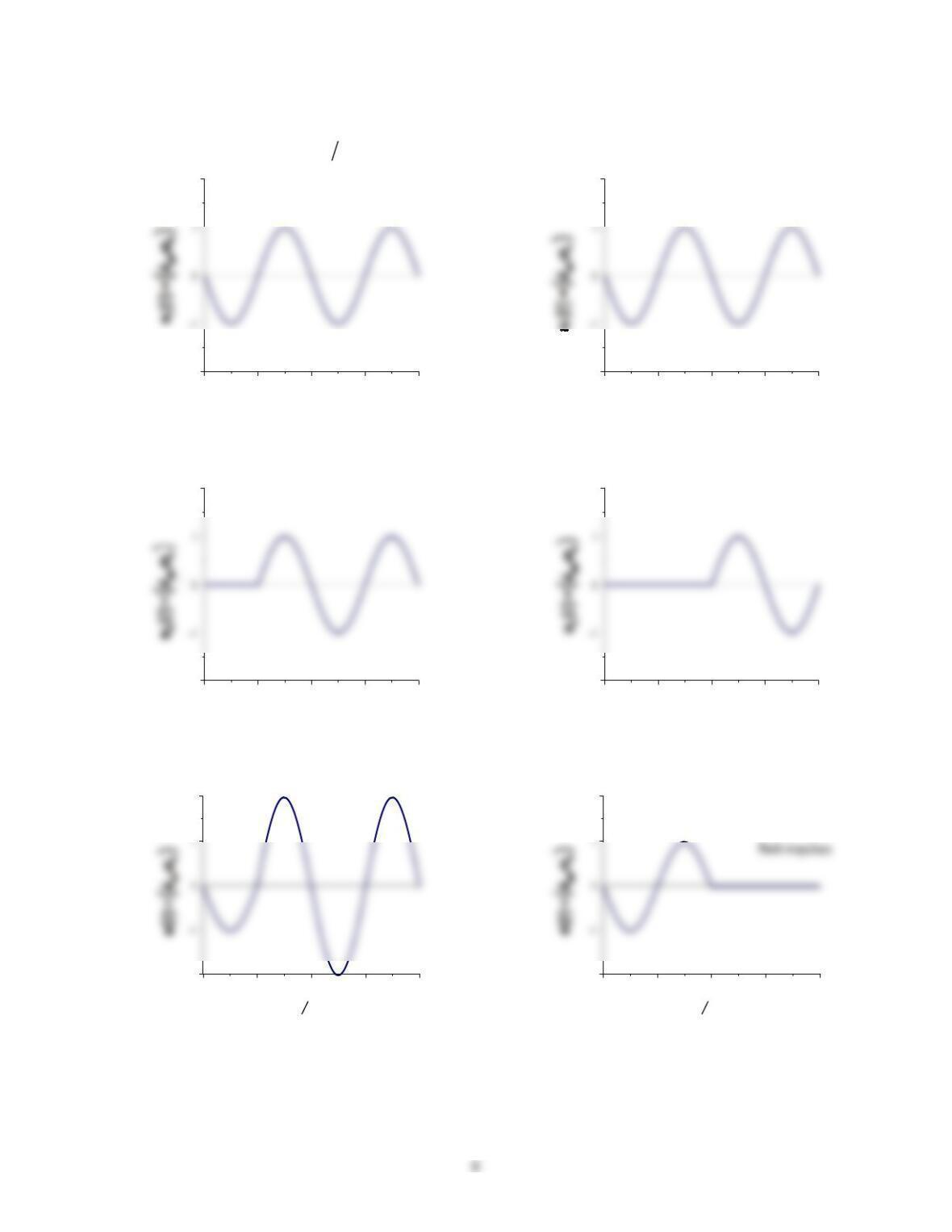
00.511.52
-2
2
tT
dn12
First impulse
00.511.52
-2
2
tT
dn1
First impulse
00.511.52
-2
2Second impulse
00.511.52
-2
2Second impulse
0 0.5 1 1.5 2
-2
2
tT
n
Both impulses
0 0.5 1 1.5 2
-2
2
tT
n
Figure P6.5c Figure P6.5d
/12
dn
tT /1
dn
tT
9
2
tT
dn
Eq. (h)
Figure P6.5e
7. Determine the overall maximum response.
From Eqs. (g) and (h), the overall maximum response
is given by
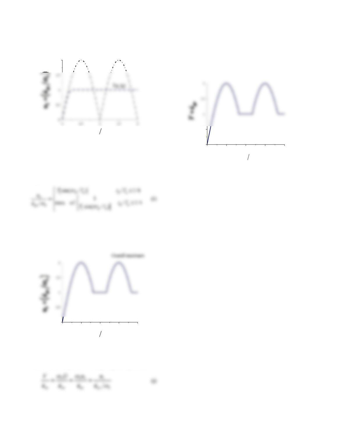
Equation (i) is plotted tT
dn
/ in Fig. P6.5f to obtain the
response spectrum.
00.511.52
0
tT
dn
Figure P6.5f
8. Determine the pseudo-velocity response spectrum.
Thus, the pseudo-velocity response spectrum for td = 0.5
sec. is given by Eq. (i) with td = 0.5 sec. This is plotted in
Fig. P6.5g.
01234
0
0.5
fT
nn
1
Figure P6.5g
10
Problem 6.6
Solution
1. Determine response to the first impulse.
ut ut
go
n1()
sin
(a)
3. Determine response to both impulses.
For 0tt
d:
d
() [sin sin ( )
go
nnd
u
ut t t t
4. Plot displacement response.
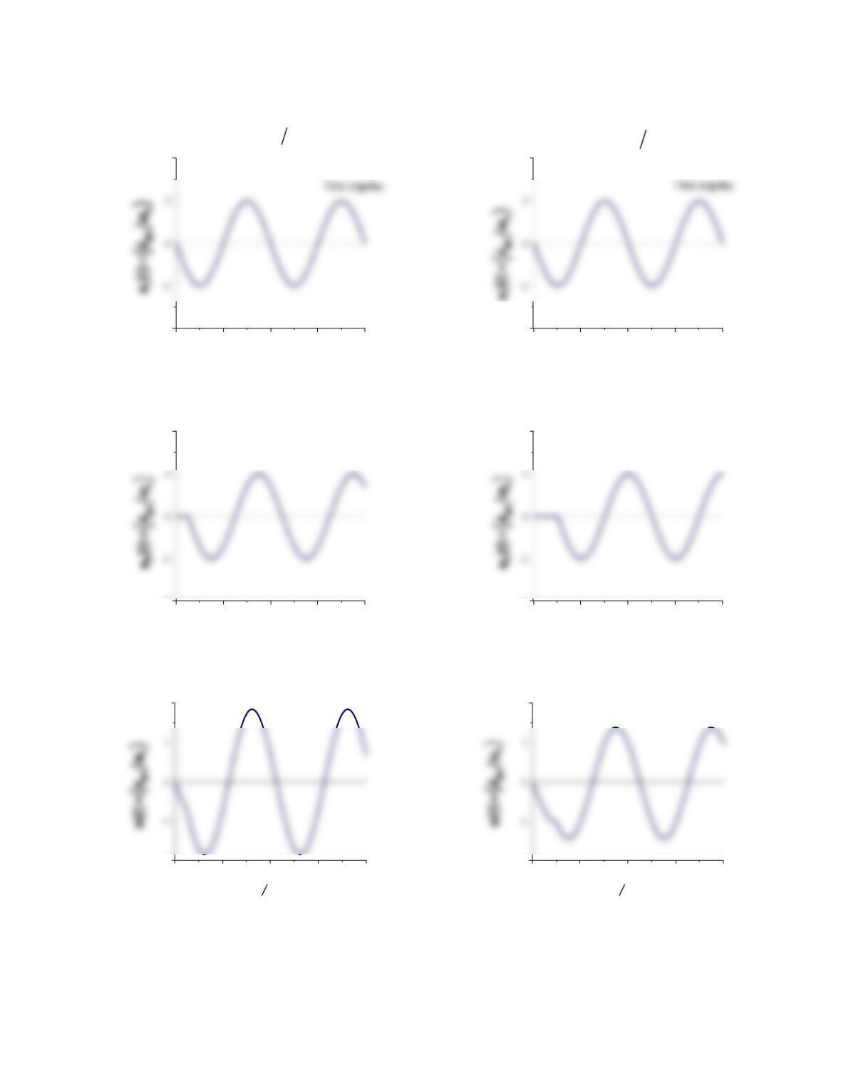
Equations (c) and (d) are plotted for tT
/
1/8, 1/4,
The number of peaks in u(t) depend on tT
dn
/; the
longer the time td between the pulses, more such peaks
Thus td must be longer than Tn/4for at least one peak
to develop during 0
tt
d.
The absolute deformation during 0
tt
d is
Equation (g) is plotted in Fig. P6.6e.
6. Determine the peak response during tt
d
.
11
00.511.52
-2
2
tT
dn
18
00.511.52
-2
2
tT
dn
14
00.511.52
-2
2Second impulse
00.511.52
-2
2
Second impulse
0 0.5 1 1.5 2
-2
2
tT
n
Both impulses
0 0.5 1 1.5 2
-2
2
tT
n
Both impulses
Figure P6.6a Figure P6.6b
/18
dn
tT /14
dn
tT
12
00.511.52
-2
2
tT
dn12
00.511.52
-2
2
tT
dn1
00.511.52
-2
2
Second impulse
00.511.52
-2
2
Second impulse
0 0.5 1 1.5 2
-2
2
tT
n
0 0.5 1 1.5 2
-2
2
tT
n
Both impulses
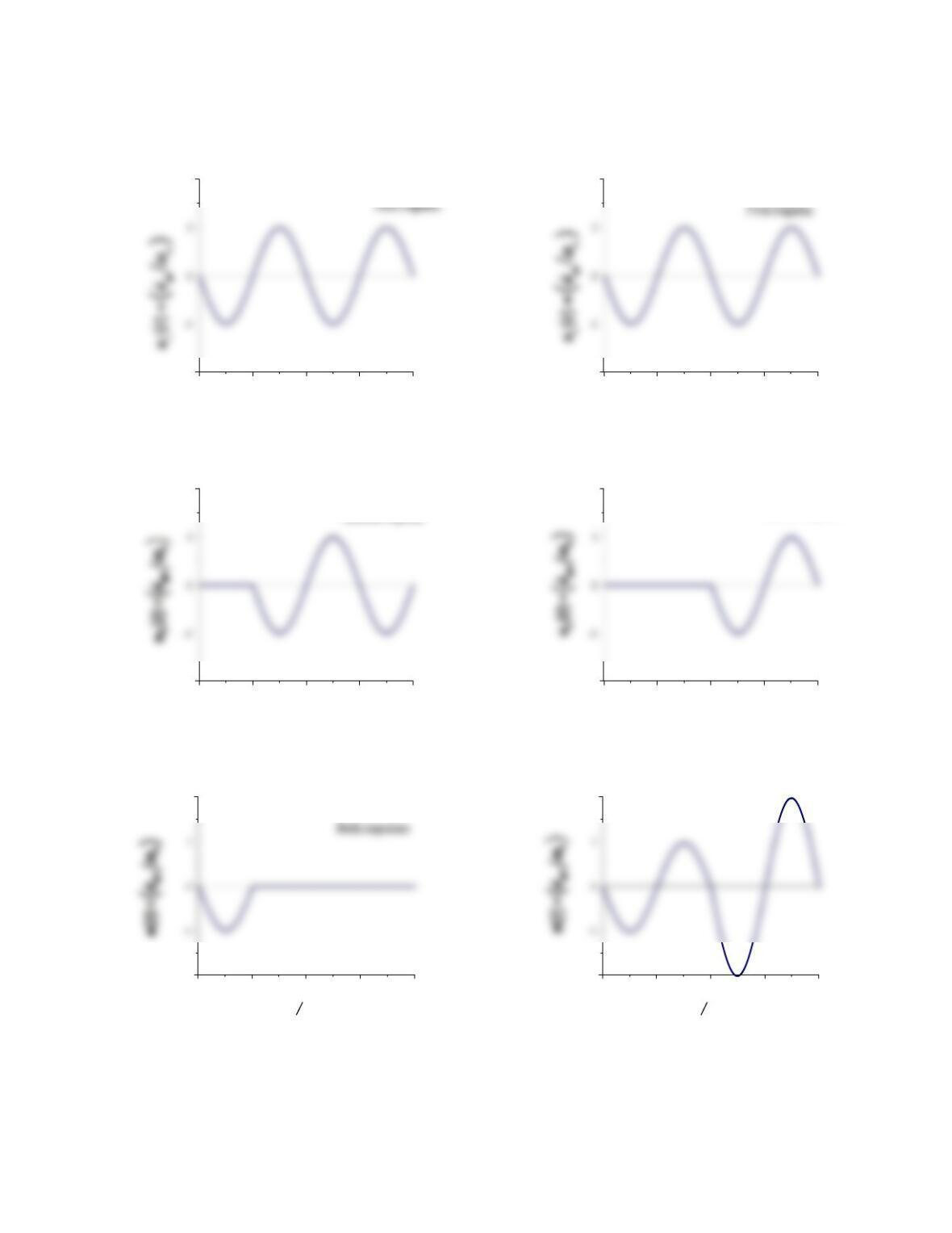
Figure P6.6c Figure P6.6d
/2
dn
tT /1
dn
tT
13
0 0.5 1 1.5 2
0.5
1.5
tT
uo()
7. Determine the overall maximum response.
From Eqs. (g) and (h), the overall maximum response
is given by
Equation (i) is plotted tT
dn
/ in Fig. P6.6f to obtain the
response spectrum.
0 0.5 1 1.5 2
0
tT
dn
Figure P6.6f
8. Determine the pseudo-velocity response spectrum.
Thus, the pseudo-velocity response spectrum for td = 0.5
01234
0
1.5
o
14
Problem 6.7
Consider harmonic ground motion ݑሷ g(t) = ݑሷ go sin (2πt/T).
(a) Derive equations for A and for ݑሷ
௧ in terms of the
natural vibration period Tn and the damping ratio ζ of the
SDF system. A is the peak value for the pseudo–
acceleration, and ݑሷ
௧ is the peak value of the true
acceleration. Consider only the steady-state response.
(b) Show that A and ݑሷ
௧ are identical for undamped
systems but different for damped systems.
(c) Graphically display the two response spectra by
plotting the normalized values A/ݑሷ go and ݑሷ
௧/ݑሷ go against
Tn/T, the ratio of the natural vibration period of the system
and the period of the excitation.
Solution
(a) The equation of motion is
The peak pseudo-acceleration AD
n
2 is
Substituting
nn
T
T
in Eq. (3.6.4) gives the true
acceleration
(b) For
0, Eqs. (c) and (d) become identical:
T
T
T
T
15
Problem 6.8
Determine the pseudo-acceleration response spectrum for
undamped systems. Plot this spectrum against td / Tn. How
will the true-acceleration response spectrum differ?
Figure P6.8
Solution
The equation of motion to be solved is
1. Determine response u(t).
Forced Vibration Phase
The response solution of Eq. (1) is
16
Free Vibration Phase
The motion is described by Eq. (4.7.3) with ut
d
()
Substituting Eq. (c) in Eq. (4.7.3) gives
ut
uTt
T
tT
tTtt
go n n d
n
dn
d
n
d
()
(/) sin cos ( )
22
1
1
22
d
tt (d)
Case 2: 1
dn
tT
Forced Vibration Phase
The forced response is now given by Eq. (3.1.13b)
Free Vibration Phase
The second equation implies that the displacement in the
forced vibration phase reaches its maximum at the end of
this phase. Substituting Eq. (f) in Eq. (4.7.3) gives
2. Plot response history.
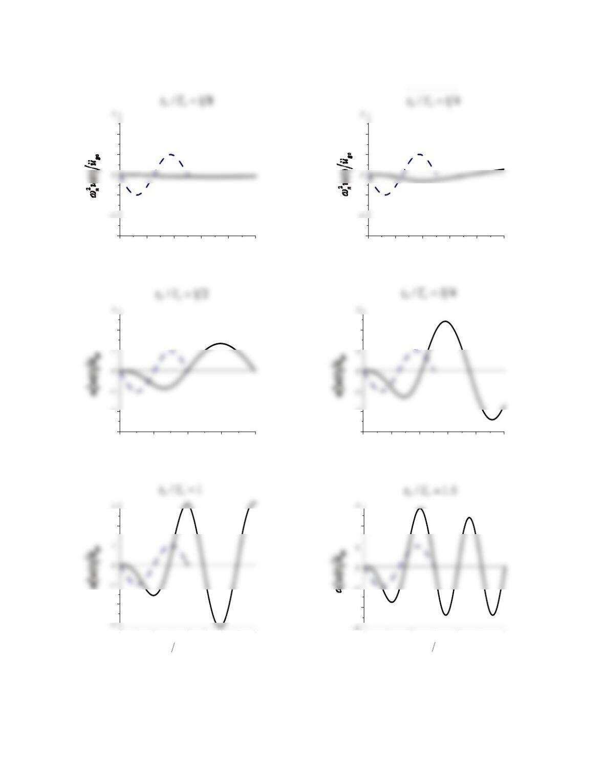
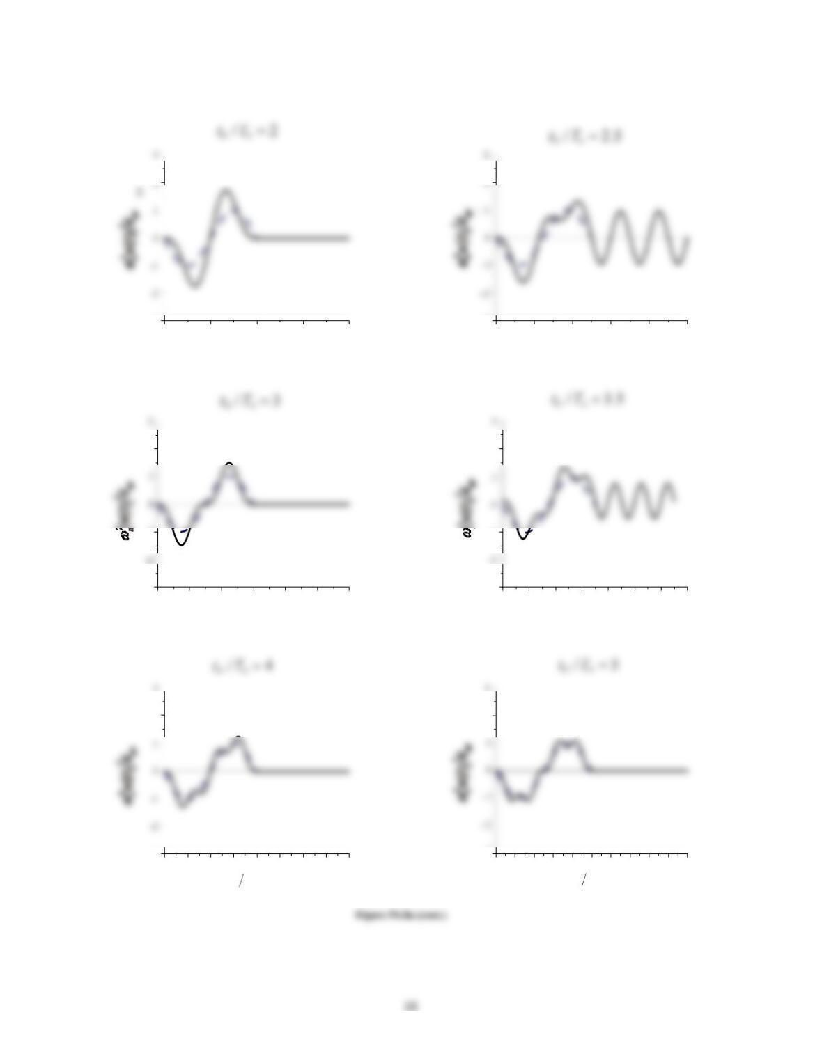
The time variation of the normalized deformation,
17
0123
tTn
2
-2
-1
3
Figure P6.8a
0 0.05 0.1 0.15 0.2 0.25
-3
-1
1
2
g
o
0 0.1 0.2 0.3 0.4 0.5
2
1
-1
-3
ngo
0 0.25 0.5 0.75 1
-3
-2
2
0 0.3 0.6 0.9 1.2 1.5
-3
2
-2
0 0.5 1 1.5 2
3
2
-2
tT
n
01234
-3
012345
-3
0123456
2
-1
-3
01234567
-3
-1
2
012345678
-3
2
3
tTn
012345678910
tTn
3
2
-3
19
During the forced vibration phase, the number of
local maxima and minima depends on td / Tn ; the longer
() (/)
tl
t
l
d01
l = 1, 2, 3... (i)
Eq. (i) into Eq. (b) and using Eq. (h) gives
2
1*
1( / )
go n d
A
uTt
excitation. If td / Tn > 1 a local minimum develops during
the ground acceleration pulse. If td / Tn > 2 more than one
For the special case of td / Tn = 1, the maximum
response during the forced vibration can be determined
from Eq. (e):
Similarly, the maximum response during free vibration
can be determined from Eq. (g):
The overall maximum response is the larger of the two
maxima determined separately for the forced and free
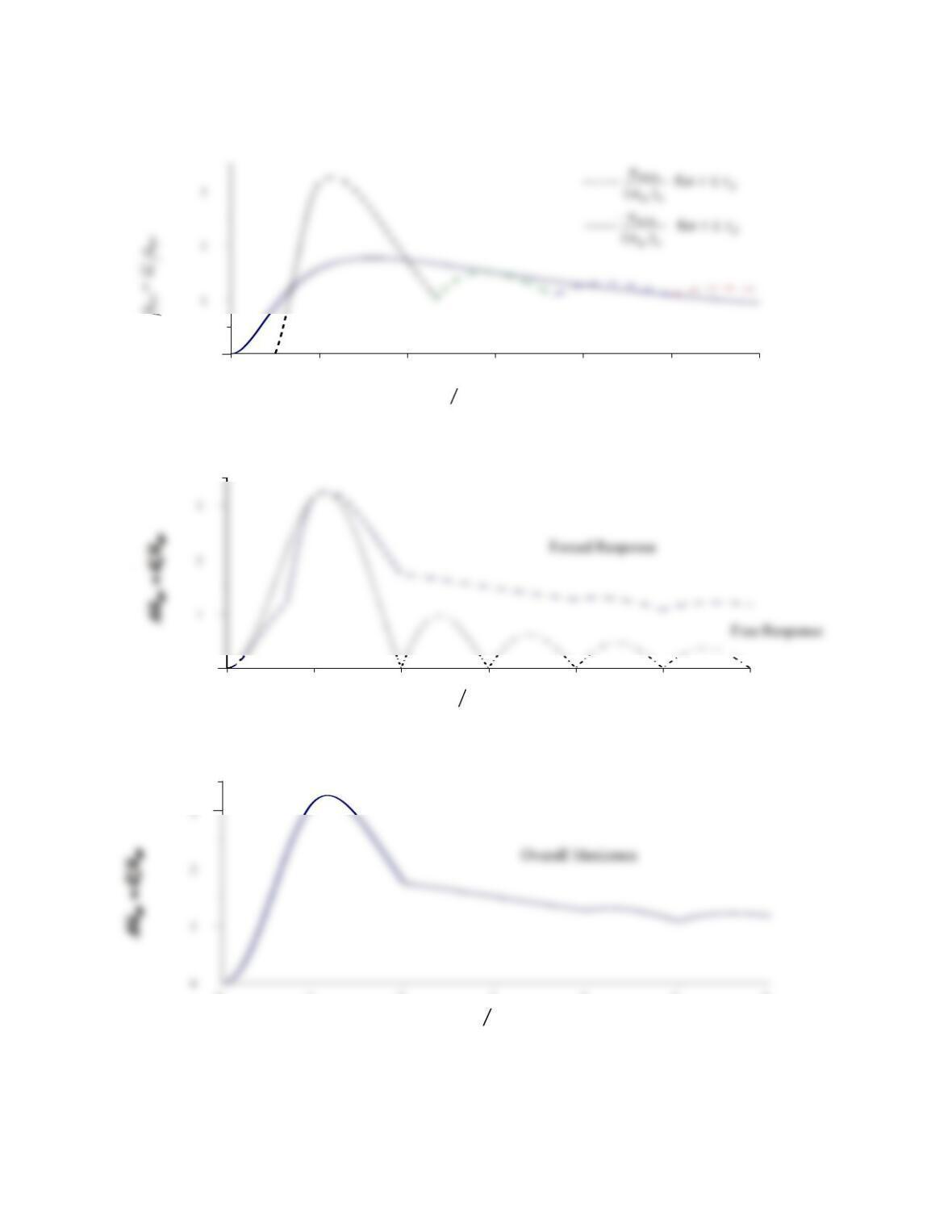
vibration phases. Figure P6.8c shows that if td Tn , the
4. True Acceleration Response Spectrum.
20
tT
dn
0123456
0
A
0123456
0
tT
dn
0123456
tT
dn
Figure P6.8b
Figure P6.8c
Figure P6.8d